Spectral Analysis

In all previous chapters, the methods fall in a big category known as time domain analysis. In this chapter, we briefly introduce spectral analysis, which tries to describe the fluctuation of time series in terms of sinusoidal behavior at various frequencies, and this is known as frequency domain analysis.
This alternative approach comes helpful when there’s no apparent seasonal period in the observed data, or when there are multiple periods. The spectral representation of a stationary time series $\{X_t\}$ decomposes it into a sum of sinusoidal components with uncorrelated random coefficients. In conjunction with this decomposition, there is a corresponding decomposition into sinusoids of the autocovariance function of $\{X_t\}$.
The tradeoff of this method is that we lose the ease of interpretation with respect to time. Instead, we’ll have to interpret the frequencies. Wavelets are similar to Fourier but contains time information, so it’s a good alternative if both time and frequencies are needed in your analysis.
Preliminaries
Often it’s more convenient to represent a function by a set of elementary functions called basis function such that all functions under study can be written as linear combinations of the elementary functions in the basis. The basis expansion of function $f(x)$ is
$$ f(x) = \sum_j a_j B_j(x) $$
where $B(x)$ is the basis function. The basis function should be determined in advance, and then the coefficients for each basis function are estimated.
One popular basis expansion is the Taylor expansion. Assuming $f(x)$ is smooth such that it possess derivatives of all orders in its domain, the Taylor expansion at $x = x_0$ is
$$ f(x) = \sum_{j=0}^\infty \frac{f^{(j)}(x_0)}{j!} (x - x_0)^j $$
where the polynomial basis is
$$ \left\{ 1, x-x_0, (x-x_0)^2, (x-x_0)^3, \cdots \right\} $$
Fourier analysis
In Fourier expansion, sines and cosines are used as the basis function. The sum of sinusoidal components with uncorrelated coefficients are given as
$$ f(\omega) = \frac{1}{2\pi} \sum_k c_k e^{ik\omega} $$
where under Euler’s identity we have
$$ e^{ik\omega} = \cos(k\omega) + i\sin(k\omega), \quad i = \sqrt{-1} $$
The complex numbers $c_k$’s are called Fourier coefficients. Their magnitudes can be measured by multiplying their conjugates to themselves:
$$ \begin{aligned} |e^{ik\omega}|^2 &= e^{ik\omega} \cdot \overline{e^{ik\omega}} = e^{ik\omega} \cdot e^{-ik\omega} \\ &= \big( \cos(k\omega) + i\sin(k\omega) \big) \big( \cos(k\omega) - i\sin(k\omega) \big) \\ &= \cos^2(k\omega) - i^2 \sin^2(k\omega) \\ &= \cos^2(k\omega) + \sin^2(k\omega) = 1 \end{aligned} $$
This tells us the magnitude for the basis function is always 1, and we’ll use this fact later. The “uncorrelated” comes from the fact that
$$ \int_{-\pi}^\pi \sin x \cos x dx = 0 $$
After using the Fourier series to represent our time series $g(t)$ by a discrete sum of complex exponentials, we can use the Fourier transform to estimate the Fourier coefficients by integral of the complex exponentials:
$$ c_k = \frac{1}{2\pi} \int_0^{2\pi} g(t) e^{-ikt} dt $$
Typically the time in our series would be discrete, so a summation instead of the integral would be used.
Simulation in R
See this post for a much better and in-depth explanation.
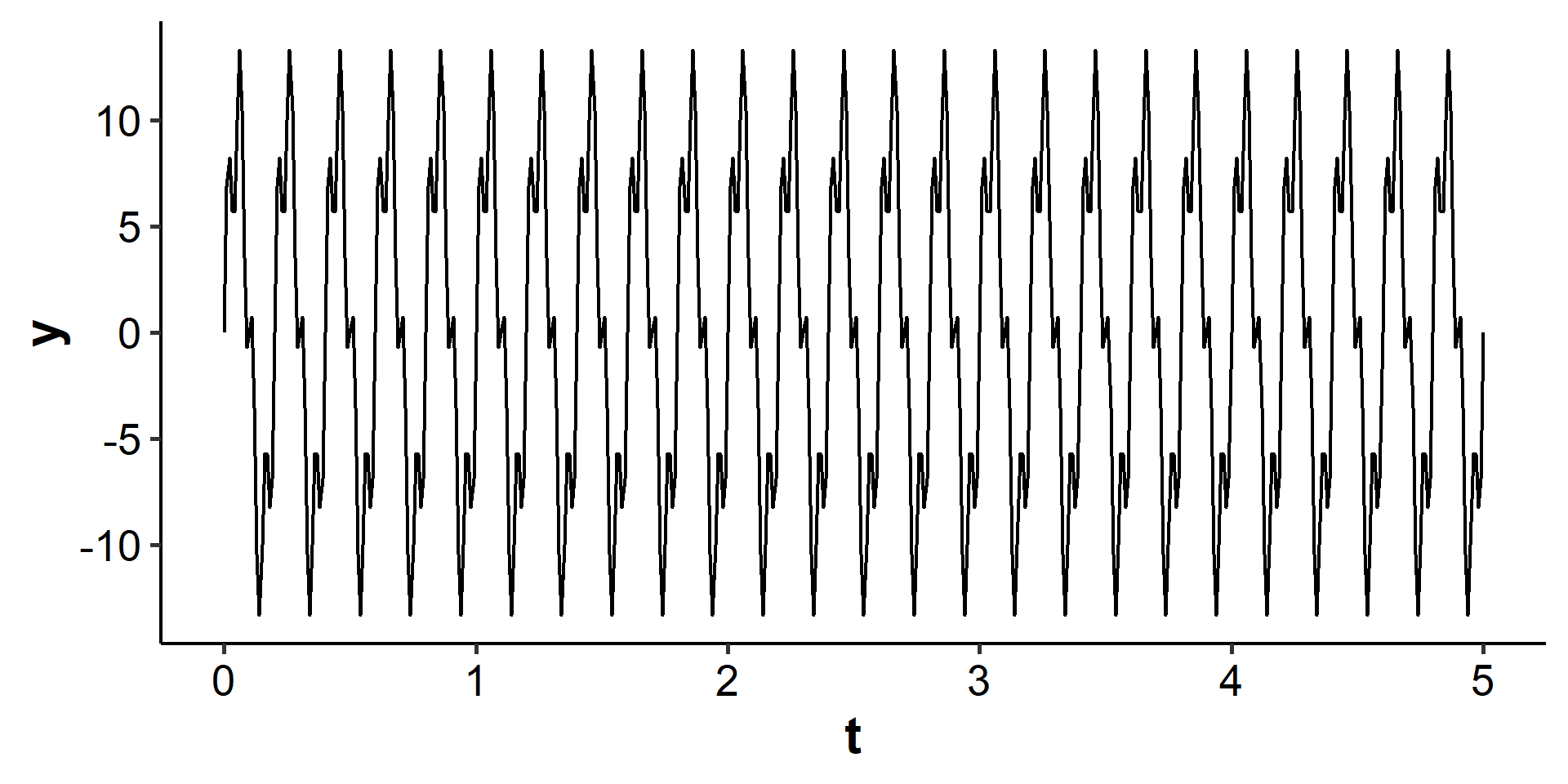
We simulate a series as the sum of two sine curves with periods of 5 and 20, respectively:
$$ y = 10\sin(5\omega t) + 4\sin(20\omega t) $$
| |
Now we can apply the Fourier transform and get the coefficients:
| |
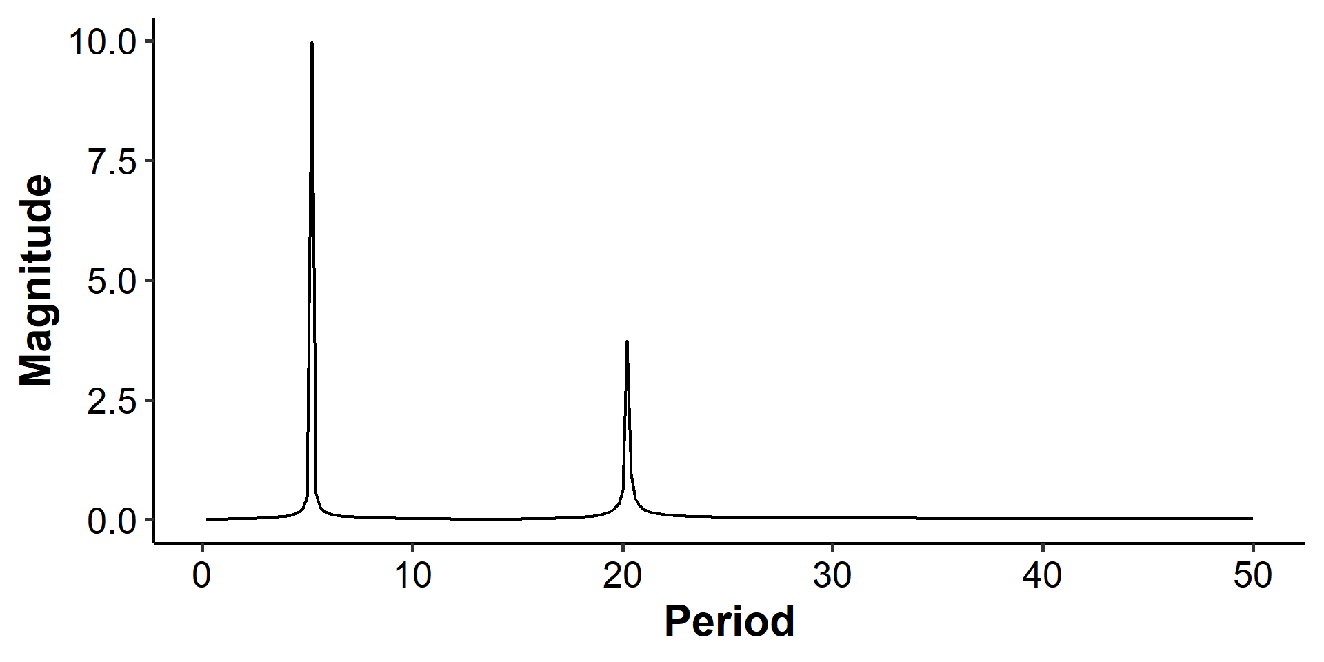
We can see two spikes at 5 and 20 with magnitudes of 10 and 4, respectively.
Spectral density
The spectral density is the counterpart of the autocovariance function in the frequency domain. Identifying the serial correlation is important in time series as it captures the autocovariance function. In the frequency domain, the Fourier transform of the autocovariance function is the spectral density.
Let $\{X_t\}$ be a stationary time series with mean zero, and its autocovariance function $\gamma$ satisfies $\sum_{k=-\infty}^\infty |\gamma(k)| < \infty$. The spectral density of $\{X_t\}$ is
$$ f(\lambda) = \frac{1}{2\pi} \sum_{k=-\infty}^\infty e^{-ik\lambda} \gamma(k), \quad -\infty < \lambda < \infty $$
The summability of $|\gamma|$ implies that the series converges absolutely.
Basic properties
$f(\lambda)$ is even, i.e. $f(\lambda) = f(-\lambda)$.
$$ f(-\lambda) = \frac{1}{2\pi} \sum_{k=-\infty}^\infty e^{ik\lambda} \gamma(k) \xlongequal{k \Rightarrow -k} \frac{1}{2\pi} \sum_{k=-\infty}^\infty e^{-ik\lambda} \gamma(-k) $$
We know that the autocovariance function is symmetric, so $\gamma(-k) = \gamma(k)$.
$f(\lambda) \geq 0$ for all $\lambda \in (-\pi, \pi]$. This also comes from the fact that $\gamma(k)$ is non-negative.
The inverse transform to get the autocovariance function from the spectral density:
$$ \gamma(k) = \int_{-\pi}^\pi e^{ik\lambda} f(\lambda) d\lambda = \int_{-\pi}^\pi \cos(k\lambda)f(\lambda)d\lambda $$
This tells us that the spectral density and the autocovariance function has a one-to-one mapping.
Examples
White noise
Let $\{X_t\} \sim WN(0, \sigma^2)$. The autocovariance function is
$$ \gamma(k) = \begin{cases} \sigma^2, & k = 0, \\ 0, & k \neq 0 \end{cases} $$
The spectral density is
$$ \begin{aligned} f(\lambda) &= \frac{1}{2\pi}\sum_{k=-\infty}^\infty e^{-ik\lambda} \gamma(k) \\ &= \frac{1}{2\pi} e^0 \gamma(0) \\ &= \frac{\sigma^2}{2\pi} \end{aligned} $$
If we find the spectral density to be constant over time, it indicates that the time series is a white noise.
MA(1)
Suppose $X_t = Z_t + \theta Z_{t-1}$. The autocovariance function is
$$ \gamma(k) = \begin{cases} (1 + \theta^2)\sigma^2, & k = 0, \\ \theta \sigma^2, & k = \pm 1, \\ 0, & \text{otherwise} \end{cases} $$
The spectral density is
$$ \begin{aligned} f(\lambda) &= \frac{1}{2\pi}\sum_{k=-\infty}^\infty e^{-ik\lambda} \gamma(k) \\ &= \frac{1}{2\pi} \left( e^{i\lambda}\gamma(-1) + e^0 \gamma(0) + e^{-i\lambda}\gamma(1) \right) \\ &= \frac{1}{2\pi} \left( \theta\sigma^2\left(e^{i\lambda} + e^{-i\lambda} \right) + (1 + \theta^2)\sigma^2 \right) \\ &= \frac{\sigma^2}{2\pi} \left( \theta(\cos\lambda + i\sin\lambda + \cos\lambda - i\sin\lambda) + 1 + \theta^2 \right) \\ &= \frac{\sigma^2}{2\pi} \left( 1 + 2\theta\cos\lambda + \theta^2 \right) \end{aligned} $$
AR(1)
Suppose $X_t = \phi X_{t-1} + Z_t$. The autocovariance function is
$$ \gamma_k = \frac{\sigma^2}{1 - \phi^2}\phi^k, \quad k = 0, 1, 2, \cdots $$
The spectral density is
$$ \begin{aligned} f(\lambda) &= \frac{1}{2\pi}\sum_{k=-\infty}^\infty e^{-ik\lambda} \gamma(k) \\ &= \frac{1}{2\pi} \left( e^0 \gamma(0) + \sum_{k=-\infty}^{-1} e^{-ik\lambda}\gamma(k) + \sum_{k=1}^\infty e^{-ik\lambda}\gamma(k) \right) \\ &= \frac{1}{2\pi} \left( \gamma(0) + \sum_{k=1}^\infty e^{ik\lambda}\gamma(-k) + \sum_{k=1}^\infty e^{-ik\lambda}\gamma(k) \right) \\ &= \frac{1}{2\pi} \left( \frac{\sigma^2}{1 - \phi^2} + \sum_{k=1}^\infty e^{ik\lambda}\frac{\sigma^2}{1 - \phi^2}\phi^k + \sum_{k=1}^\infty e^{-ik\lambda} \frac{\sigma^2}{1 - \phi^2}\phi^k \right) \\ &= \frac{\sigma^2}{2\pi(1 - \phi^2)} \left( 1 + \sum_{k=1}^\infty \left(\phi e^{i\lambda}\right)^k + \sum_{k=1}^\infty \left(\phi e^{-i\lambda}\right)^k \right) \end{aligned} $$
Recall the sum of the infinite geometric series:
$$ \sum_{k=1}^\infty a^k = \frac{a}{1 - a} = \frac{\text{first term}}{1 - \text{common factor}} $$
So,
$$ \begin{aligned} f(\lambda) &= \frac{\sigma^2}{2\pi(1 - \phi^2)} \left( 1 + \frac{\phi e^{i\lambda}}{1 - \phi e^{i\lambda}} + \frac{\phi e^{-i\lambda}}{1 - \phi e^{-i\lambda}} \right) \\ &= \frac{\sigma^2}{2\pi(1 - \phi^2)} \cdot \frac{(1 - \phi e^{i\lambda})(1 - \phi e^{-i\lambda}) + \phi e^{i\lambda}(1 - \phi e^{-i\lambda}) + \phi e^{-i\lambda}(1 - \phi e^{i\lambda})}{(1 - \phi e^{i\lambda})(1 - \phi e^{-i\lambda})} \end{aligned} $$
See that
$$ \begin{aligned} (1 - \phi e^{i\lambda})(1 - \phi e^{-i\lambda}) &= 1 - \phi e^{-i\lambda} - \phi e^{i\lambda} + \phi^2 e^{i\lambda} e^{-i\lambda} \\ &= 1 - \phi(e^{-i\lambda} + e^{i\lambda}) + \phi^2 |e^{i\lambda}|^2 \\ &= 1 - \phi(\cos\lambda - i\sin\lambda + \cos\lambda + i\sin\lambda) + \phi^2 \\ &= 1 - 2\phi\cos\lambda + \phi^2 \end{aligned} $$
So the spectral density is
$$ \begin{aligned} f(\lambda) &= \frac{\sigma^2}{2\pi(1 - \phi^2)} \cdot \frac{1 - \phi e^{-i\lambda} - \phi e^{i\lambda} + \phi^2e^{i\lambda}e^{-i\lambda} + \phi e^{i\lambda} - \phi^2 e^{i\lambda}e^{-i\lambda} + \phi e^{-i\lambda} - \phi^2 e^{i\lambda}e^{-i\lambda} }{1 - 2\phi\cos\lambda + \phi^2} \\ &= \frac{\sigma^2}{2\pi(1 - \phi^2)} \cdot \frac{1 - \phi^2}{1 - 2\phi\cos\lambda + \phi^2} \\ &= \frac{\sigma^2}{2\pi(1 - 2\phi\cos\lambda + \phi^2)} \end{aligned} $$
We can see that the density is large for low frequencies, and small for high frequencies.
ARMA(1, 1)
We have $\phi(B) = 1 - \phi B$ and $\theta(B) = 1 + \theta B$. The spectral density is
$$ \begin{aligned} f(\lambda) &= \frac{\sigma^2|\theta(e^{-i\lambda})|^2}{2\pi |\phi(e^{-i\lambda})|^2} \\ &= \frac{\sigma^2}{2\pi} \cdot \frac{(1 + \theta e^{-i\lambda})(1 + \theta e^{i\lambda})}{(1 - \phi e^{-i\lambda})(1 - \phi e^{i\lambda})} \\ &= \frac{\sigma^2}{2\pi} \cdot \frac{1 + 2\theta\cos\lambda + \theta^2}{1 - 2\phi\cos\lambda + \phi^2} \end{aligned} $$
Calculation in R
The arma.spec() function from the astsa R package could be used to get the spectral density for different ARMA models.
| |
Note that the spectrum function is defined with a scaling factor of $\frac{1}{freq(x)}$ and returns a spectral density over the range $(-\frac{freq(x)}{2}, \frac{freq(x)}{2}]$. The more common scaling factors are $2\pi$ or $1$, and the ranges are $(-0.5, 0.5]$ or $(-\pi, \pi]$, respectively.
Periodogram
If $\{X_t\}$ is a stationary time series with autocovariance function $\gamma$ and spectral density $f$, then the sample autocovariance function $\hat\gamma$ of the observations $\{x_1, \cdots, x_n\}$ can be regarded as a sample analogue of $\gamma$. Following the same logic, the periodogram $I_n$ of the observations can be regarded as a sample analogue of $2\pi f$.
The periodogram of $\{x_1, \cdots, x_n\}$ is
$$ I_n(\lambda) = \frac{1}{n} \left| \sum_{t=1}^n x_t e^{-it\lambda} \right|^2 $$
Let $\omega_k = \frac{2\pi k}{n}$ where $k$ is any integer between $-\frac{n-1}{2}$ and $\frac{n}{2}$. This is called the Fourier frequencies associated with sample size $n$. If $x_1, \cdots, x_n$ are real numbers, and $\omega_k$ is any of the non-zero Fourier frequencies in $(-\pi, \pi]$, then
$$ I_n(\omega_k) = \sum_{|h| < n} \hat\gamma(h)e^{-ih\omega_k} $$
where $\hat\gamma(h)$ is the sample autocovariance function of $x_1, \cdots, x_n$.
The periodogram can be used to identify the dominant periods (or frequencies) of a time series. It’s helpful for identifying the cyclical behavior in a series, particularly when the cycles are not related to the commonly encountered monthly or quarterly seasonality.
Sunspot data example
We use the sunspot.year data to explain how to interpret a periodogram. The dataset contains yearly numbers of sunspots from 1700 to 1988 (rounded to one digit).
| |
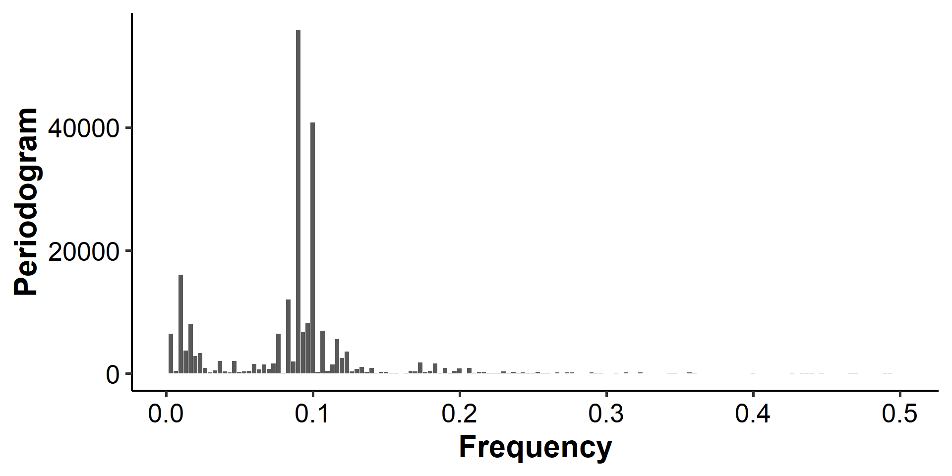
The dominant peak occurs somewhere around a frequency of 0.091. This corresponds to a period of about $\frac{1}{0.09} \approx 11$ time periods. Thus, there appears to be a dominant periodicity of about 11 years in sunspot activity (because the observations are taken yearly).
We’re also ignoring the spike(s) around frequency zero, because the low-frequency behavior corresponds to trends rather than seasonal/periodical components.
This can be found with
x$freq[which.max(x$spec)]. ↩︎
| Nov 02 | Decomposition and Smoothing Methods | 14 min read |
| Oct 13 | Seasonal Time Series | 17 min read |
| Oct 09 | Variability of Nonstationary Time Series | 13 min read |
| Oct 05 | ARIMA Models | 9 min read |
| Sep 30 | Mean Trend | 13 min read |