Model Fitting and Forecasting

In the previous chapter, we learned about the characteristics of AR, MA and ARMA processes and generated data from these known models. In real data analysis, we only have the data and don’t know the true underlying model. Our workflow typically follows:
- Time series plot: stationarity (mean, variance trend, seasonal pattern).
- Identification of serial correlation using ACF and PACF.
- Model fitting.
- Model diagnosis.
- Choose the best model by the AIC/BIC (minimize), prediction ability (MAPE), and the number of parameters.
Model identification
In model identification, we need to find appropriate models for a given observed series. The model is tentative, and is subject to revision later on in the analysis.
Usually the first step is plotting the data and see if it looks stationary. If it seems stationary, we try to identify serial correlation using the ACF and the PACF. The characteristics of the ACF and PACF are given in the table below.
| Process | ACF | PACF |
|---|---|---|
| $AR(p)$ | Tails off as exponential decay | Cuts off after lag $p$ |
| $MA(q)$ | Cuts off after lag $q$ | Tails off as exponential decay |
| $ARMA(p, q)$ | Tails off after lag $q-p$ | Tails off after lag $p-q$ |
Information criteria
For each model, we start from the lowest-order model1 and look at the residuals. If we observe prominent spikes in either the ACF or the PACF, we then sequentially increase the order. Otherwise, we keep the model as simple as possible.
Recall the definition of the likelihood function. It’s a measure of how likely the parameter estimates are. The problem with likelihood functions is that they always increase as we use more parameters. We introduce information criteria to deal with the trade-off between the goodness of fit of the model and the simplicity of the model, i.e. risks of overfitting and underfitting.
Two popular criteria to choose the best model are the AIC (Akaike information criterion) and the BIC (Bayesian information criterion):
$$ \begin{gathered} AIC(l) = \ln(\tilde{\sigma}_l^2) + \frac{2(l + 1)}{T} \\ BIC(l) = \ln(\tilde{\sigma}_l^2) + \frac{(l + 1)\ln(T)}{T} \end{gathered} $$
where $\tilde{\sigma}_l^2$ is the maximum likelihood estimate of $\sigma^2$, $T$ is the sample size, and $l$ is the number of parameters2. We select $l \in \{0, 1, \cdots, P\}$ that minimizes the AIC or the BIC. Essentially we’re trying to minimize the negative log-likelihood considering the number of parameters.
To determine whether or not to include the intercept in the model, we may use a one-sample t-test with hypotheses $H_0: \mu = 0$ vs. $H_1: \mu \neq 0$, and the test statistic is
$$ t = \frac{\bar{X}}{\sqrt{\frac{Var(X_t)}{T}}} \approx N(0, 1) $$
Here we’re essentially investigating $\mu = E(X_t)$.
AR
In this section, we’re going to use the AR(1) process as an example to introduce parameter estimation and model diagnostics methods.
Estimation
The common methods to estimate parameters are MME (method of moments estimation), LSE (least squares estimation) and MLE (maximum likelihood estimation), where the MLE has a distribution assumption as the likelihood function requires the PDF. In many cases the three methods are very similar, and the MLE performs better in complex cases.
Method of moments
For an AR(1) process with mean 0, the model is given by
$$ X_t = \phi X_{t-1} + Z_t $$
where $Z_t: WN(0, \sigma^2)$. The parameters to estimate are $\phi$ and $\sigma^2$.
$$ \begin{gathered} \phi = \frac{\gamma_X(1)}{\gamma_X(0)}, && \sigma^2 = (1 - \phi^2)\gamma_X(0) \\ \hat\phi = \frac{\sum_{t=1}^{T-1} X_t X_{t+1}}{\sum_{t=1}^T X_t^2}, && \hat\sigma^2 = (1 - \hat\phi^2) \cdot \frac{1}{T}\sum_{t=1}^T X_t^2 \end{gathered} $$
For an AR(1) model with mean $\mu$, the model is
$$ X_t - \mu = \phi(X_{t-1} = \mu) + Z_t $$
so we have one more parameter to estimate. The formulae are very similar:
$$ \begin{gathered} \hat\mu = \bar{X} \\ \hat\phi = \frac{\sum_{t=1}^{T-1} (X_t - \bar{X})(X_{t+1} - \bar{X})}{\sum_{t=1}^T (X_t - \bar{X})^2} \\ \hat\sigma^2 = (1 - \hat\phi^2) \cdot \frac{1}{T}\sum_{t=1}^T (X_t - \bar{X})^2 \end{gathered} $$
For an AR(2) model with mean 0:
$$ X_t = \phi_1 X_{t-1} + \phi_2 X_{t-2} + Z_t, $$
we may use the Yule-Walker equation to get
$$ \begin{gathered} \rho_X(1) = \phi_1 + \phi_2 \rho_X(1) \\ \rho_X(2) = \phi_1 \rho_X(1) + \phi_2 \end{gathered} $$
which allows us to express $\phi_1$ and $\phi_2$ using the autocorrelation functions:
$$ \begin{gathered} \phi_2 = \frac{\rho_X(2) - \rho_X(1)^2}{1 - \rho_X(1)^2} \\ \phi_1 = \frac{\rho_X(1) - \rho_X(1) \rho_X(2)}{1 - \rho_X(1)^2} \end{gathered} $$
We know that
$$ \hat\rho_X(k) = \frac{\sum_{t=1}^{T_k} X_t X_{t+k}}{\sum_{t=1}^T X_t^2}, $$
therefore, $\hat\phi_1$ and $\hat\phi_2$ can both be expressed using $\hat\rho_X(1)$ and $\hat\rho_X(2)$. The estimator for $\sigma^2$ can be found from the equation for $Var(X_t)$:
$$ \hat\sigma^2 = \left(1 - \hat\phi_1 \hat\rho_X(1) - \hat\phi_2 \hat\rho_X(2) \right) \cdot \frac{1}{T}\sum_{t=1}^T X_t^2 $$
Least squares
For the AR(1) process
$$ X_t - \mu = \phi(X_{t-1} - \mu) + Z_t, $$
the sum of squared errors is
$$ SSE = \sum_{t=1}^T Z_t^2 = \sum_{t=2}^T (X_t - \delta - \phi X_{t-1})^2 $$
To minimize the conditional sum of squares:
$$ \begin{gathered} s^*(\phi, \delta) = \sum_{t=2}^T \left( (X_t - \mu) - \phi(X_{t-1} - \mu) \right)^2 \\ \hat\mu \approx \bar{X} \\ \hat\phi = \frac{\sum_{t=2}^T (X_t - \bar{X})(X_{t-1} - \bar{X})}{\sum_{t=2}^T (X_{t-1} - \bar{X})^2} \\ \hat\sigma^2 = \frac{1}{T-3}\sum_{t=2}^T \left( (X_t - -\bar{X}) - \hat\phi(X_{t-1} - \bar{X}) \right)^2 \end{gathered} $$
Maximum likelihood estimation
Assuming $Z_t \overset{i.i.d.}{\sim} N(0, \sigma^2)$, we want to find $(\mu, \phi, \sigma^2)$ which minimizes
$$ L(\phi, \mu, \sigma^2) - \prod_{t=2}^T \frac{1}{\sqrt{2\pi}\sigma}\exp \left\{ -\frac{((X_t - \mu) - \phi(X_{t-1} - \mu))^2}{2\sigma^2} \right\} $$
By partial derivatives we’ll get
$$ \begin{gathered} \hat\mu = \frac{1}{T-1}\sum_{t=2}^T X_{t-1} \approx \bar{X} \\ \hat\phi = \frac{\sum_{t=2}^T (X_t - \hat\mu)(X_{t-1} - \hat\mu)}{\sum_{t=2}^T (X_{t-1} - \hat\mu)^2} \\ \hat\sigma^2 = \frac{1}{T-1}\sum_{t=2}^T \left( (X_t - \hat\mu) - \hat\phi(X_{t-1} - \hat\mu) \right)^2 \end{gathered} $$
Model diagnostics
To check the assumption that $Z_t \sim N(0, \sigma^2)$, we perform the white noise check.
The standardized residuals (innovations) are
$$ e_t = \frac{X_t - \tilde{X}_t^{t-1}}{\sqrt{\hat{V} \left(X_t - \tilde{X}_t^{t-1} \right)}} $$
where $\tilde{X}_t^{t-1}$ is the forecast for time $t$ using information up to time $t-1$, and $\hat{V}(X_t - \tilde{X}_t^{t-1})$ is the estimate of $Var(X_t - \tilde{X}_t^{t-1})$. If the correct model is chosen, these standardized residuals should approximately follow $N(0, 1)$. Thus, we’d expect about 95% of them to fall within $\pm 2$ and about 99% to fall within $\pm 3$. Standardized residuals falling outside of this range indicate an incorrect model may have been chosen.
We should also check the ACF/PACF of the standardized residuals. If the residuals are really i.i.d. normal, there should only be a spike at lag 0 and all the other lags should fall within the band:
$$ \hat\rho(k) \pm \frac{2}{\sqrt{T}} $$
This could be tested using the Ljung-Box test (Portmanteau test), which tests if any of a group of autocorrelations of a time series are different from zero. The hypotheses are
$$ \begin{gathered} H_0: \rho(1) = \cdots = \rho(m) = 0 \text{ vs.} \\ H_1: \rho(i) \neq 0 \text{ for at least one } i. \end{gathered} $$
The test statistic is
$$ Q(m) = T(T+2) \sum_{k+1}^m \frac{\hat\rho(k)^2}{T-k} \approx \chi^2(m - \text{ number of parameters in the model}) $$
Usually we have $m \approx \log(T)$ where $T$ is the number of timepoints. For AR(1) with mean 0, there’s only one parameter3 $\phi$ so the degrees of freedom is $m-1$. For AR(1) with mean $\mu$, the d.f. is $m-2$.
Simulation in R
We use the following code to simulate an AR(1) process with $\phi = 0.5$ and $n = 100$.
| |
The estimated parameter $\hat\phi = 0.5377$ and the estimated $\hat\sigma^2 = 0.8398$. Thus the fitted model is
$$ X_t = 0.5377 X_{t-1} + Z_t, \quad Z_t \sim N(0, 0.8398) $$
Next we check the assumptions of the fitted model. The tsdiag() function generates three diagnosis plots: the standardized residuals plot, the ACF of the residuals, and the p-values for the Ljung-Box statistic. The gof.lag parameter gives the maximum number of lags for the test.
Alternatively, we may use functions from other packages to model (forecast::auto.arima) and plot (ggfortify::ggtsdiag) the data4.
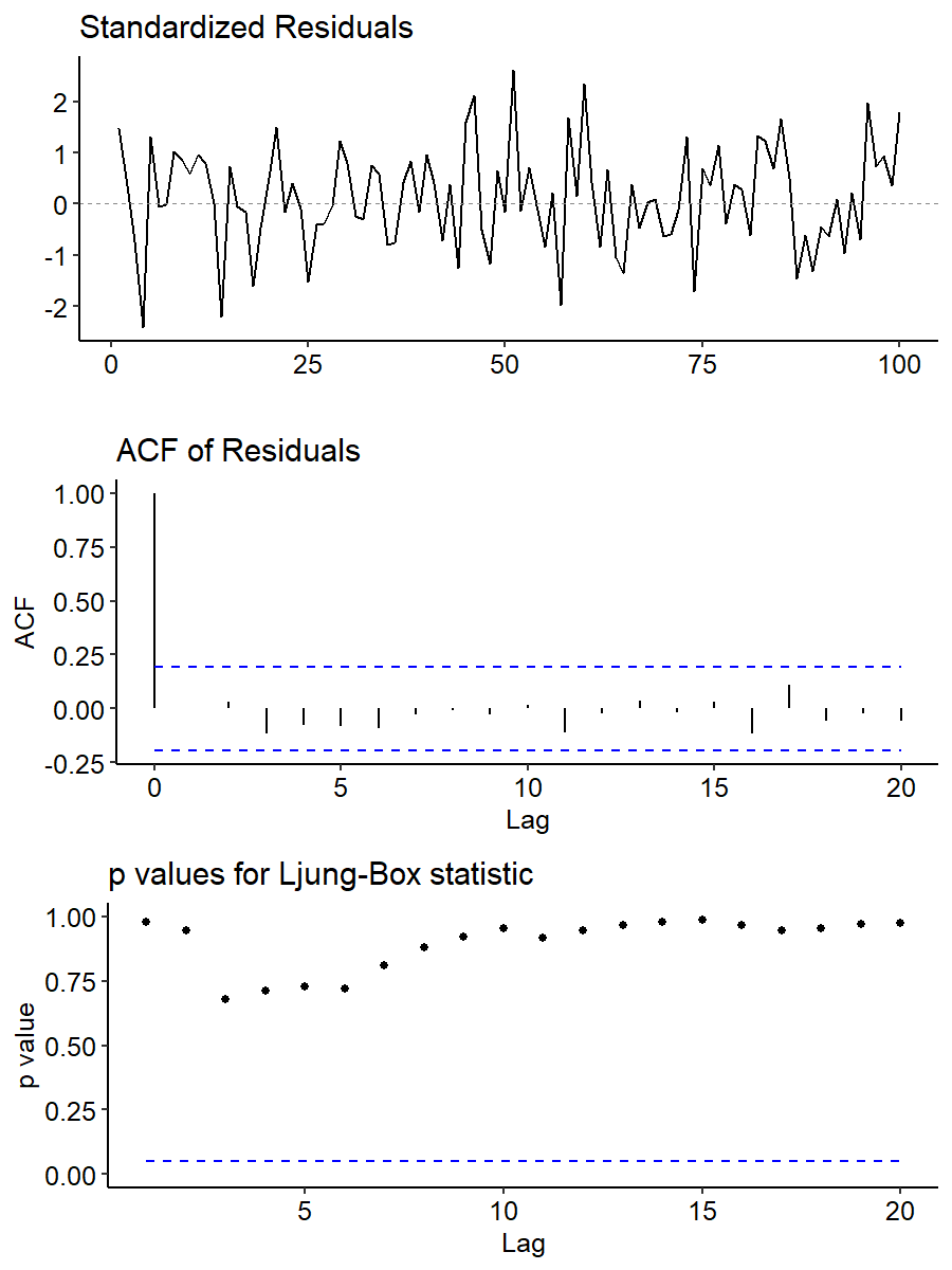
The standardized residuals plot is centered around zero, and there’s no specific patterns with most values falling within $\pm 2$. For the ACF plot, everything falls within the bands except for lag 0, indicating no serial correlations. Finally, the p-values for the Ljung-Box statistic are all very high, meaning the none of the $H_0$’s can be rejected and there’s no evidence at any lag that $\rho = 0$. Overall we observe no signs of violation of the assumptions.
We can also perform the Ljung-Box test using the Box.test() function. Here’s an example for lag 3:
| |
Note we specified fitdf = 1 to subtract 1 from the degrees of freedom to get the correct number. The d.f. should be 2, which is $m$ (lag 3) minus the number of parameters in AR(1). This is why the computed p-value of 0.469 doesn’t seem to match the value in the figure5.
Forecasting
After we’ve confirmed that the fitted model is good enough, the next step is predicting future values. Recall how prediction was done in multiple regression. Suppose the model is
$$ Y_i = \beta_0 + \beta_1 X_{i1} + \cdots + \beta_p X_{ip} + \epsilon_i, \quad \epsilon_i \overset{i.i.d.}{\sim} N(0, \sigma^2) $$
where we have $p$ predictor variables and $n$ observations. We have
$$ E\left( Y_i \mid X_{i1}, \cdots, X_{ip} \right) = \beta_0 + \beta_1 X_{i1} + \cdots + \beta_p X_{ip} $$
Now if a new observation $(x_1, \cdots, x_p)$ comes in, we make the prediction by
$$ \hat{y} = \hat\beta_0 + \hat\beta_1 x_1 + \cdots + \hat\beta_p x_p = \hat{E}(Y \mid x_1, \cdots, x_p) $$
Time series forecasting
Given the past data up to timepoint $t$ ($X_t, X_{t-1}, \cdots, X_1$), the $k$ time ahead forecast (or lag $k$ forecast) at time $t$ is
$$ X_t(k) = E(X_{t+k} \mid X_t, X_{t-1}, \cdots, X_1) $$
For example, predicting $X_{101}$ given $X_1, \cdots, X_{100}$ is 1 time ahead forecast at time 100.
The forecasting error for this point estimation is
$$ e_t(k) = X_{t+k} - X_t(k) $$
We need this quantity to calculate the standard error $Var(e_t(k))$ and construct confidence intervals:
$$ \text{point estimate } \pm z_\frac{\alpha}{2} \cdot S.E. $$
The AR(1) model is
$$ X_t - \mu = \phi(X_{t-1} - \mu) + Z_t, \quad Z_t \overset{i.i.d.}{\sim}N(0, \sigma^2) $$
and we have $E(X_t) = \mu$. Let $Y_t = X_t - \mu$, then $E(Y_t) = 0$, and the AR(1) model with mean 0 would be
$$ Y_t = \phi Y_{t-1} + Z_t $$
The prediction for $X_t$ can be simply derived from $Y_t$ as their difference is a constant term.
Lag 1 forecast
The lag 1 forecast is
$$ \begin{aligned} Y_t(1) &= E(Y_{t+1} \mid Y_t, Y_{t-1}, \cdots, Y_1) \\ &= E(\phi Y_t + Z_{t+1} \mid Y_t, Y_{t-1}, \cdots, Y_1) \\ &= \phi Y_t + E(Z_{t+1} \mid Y_t, Y_{t-1}, \cdots, Y_1) \\ &= \phi Y_t + E(Z_{t+1}) = \phi Y_t \\ \widehat{Y_t(1)} &= \hat\phi Y_t \\ X_t(1) - \mu &= \phi(X_t - \mu) \\ \widehat{X_t(1)} &= \hat\mu + \hat\phi(X_t - \hat\mu) \end{aligned} $$
The forecasting error for $X_t$ and $Y_t$ are the same because their only difference is a constant term:
$$ \begin{aligned} e_t(1) &= Y_{t+1} - Y_t(1) \\ &= \phi Y_t + Z_{t+1} - \phi Y_t \\ &= Z_{t+1} \end{aligned} $$
From this we have
$$ Var(e_t(1)) = Var(Z_{t+1}) = \sigma^2, $$
so the $100(1-\alpha)\%$ prediction interval for $Y_{t+1}$ is
$$ \widehat{Y_t(1)} \pm z_{\frac{\alpha}{2}} \cdot \sqrt{\widehat{Var}(e_t(1))} = \hat\phi Y_t \pm z_\frac{\alpha}{2} \cdot \hat\sigma $$
The $100(1-\alpha)\%$ prediction interval for $X_{t+1}$ is
$$ \widehat{X_t(1)} \pm z_{\frac{\alpha}{2}} \cdot \sqrt{\widehat{Var}(e_t(1))} = \hat\mu + \hat\phi (X_t - \hat\mu) \pm z_\frac{\alpha}{2} \cdot \hat\sigma $$
Lag 2 forecast
The 2 time ahead forecast is
$$ \begin{aligned} Y_t(2) &= E(Y_{t+2} \mid Y_t, Y_{t-1}, \cdots, Y_1) \\ &= E(\phi Y_{t+1} + Z_{t+2} \mid Y_t, Y_{t-1}, \cdots, Y_1) \\ &= \phi E(Y_{t+1} \mid Y_t, Y_{t-1}, \cdots, Y_1) + E(Z_{t+2} \mid Y_t, Y_{t-1}, \cdots, Y_1) \\ &= \phi Y_t(1) + 0 \\ &= \phi^2 Y_t \end{aligned} $$
This gives us
$$ \begin{gathered} \hat{Y}_t(2) = \hat\phi^2 Y_t \\ \hat{X}_t(2) = \hat\mu + \hat\phi^2(X_t - \hat\mu) \end{gathered} $$
The forecasting error is
$$ \begin{aligned} e_t(2) &= Y_{t+2} - Y_t(2) \\ &= \phi Y_{t+1} + Z_{t+2} - \phi^2 Y_t \\ &= \phi (\phi Y_t + Z_{t+1}) + Z_{t+2} - \phi^2 Y_t \\ &= \phi Z_{t+1} + Z_{t+2} \end{aligned} $$
Thus,
$$ \begin{aligned} Var(E_t(2)) &= Var(\phi Z_{t+1} + Z_{t+2}) \\ &= \phi^2 \sigma^2 + \sigma^2 = (1 + \phi^2)\sigma^2 \end{aligned} $$
and the $100(1-\alpha)\%$ prediction interval for $Y_t(2)$ is
$$ \hat\phi^2 \pm Z_\frac{\alpha}{2} \sqrt{(1 + \hat\phi^2)\hat\sigma^2} $$
The $100(1-\alpha)\%$ prediction interval for $X_t(2)$ is
$$ \hat\mu + \hat\phi^2 (X_t - \hat\mu) \pm Z_\frac{\alpha}{2} \sqrt{(1 + \hat\phi^2)\hat\sigma^2} $$
General case
In general, the $k$ time ahead forecast, forecasting error and $100(1-\alpha)\%$ prediction interval at time $T$ are given by
$$ \begin{gathered} X_t(k) = E(X_{t+k} \mid X_t, X_{t-1}, \cdots, X_1) = \phi^k(X_t - \mu) + \mu \\ e_t(k) = X_{t+k} - X_t(k) = Z_{t+k} + \phi Z_{t+k-1} + \phi^2 Z_{t+k-2} + \cdots + \phi^{k-1}Z_{t+1} \\ Var(e_t(k)) = \sigma^2 \cdot \frac{1 - \phi^{2k}}{1 - \phi^2} \\ \hat{X}T(k) = \hat\mu + \hat\phi^k (X_T - \hat\mu), \quad \hat\mu + \hat\phi^k (X_T - \hat\mu) \pm Z{\frac{\alpha}{2}} \sqrt{\frac{1 - \phi^{2k}}{1 - \phi^2}} \hat\sigma \end{gathered} $$
Calculation in R
To predict future values using our fitted model x.fit, we may use the built-in predict() function in R.
| |
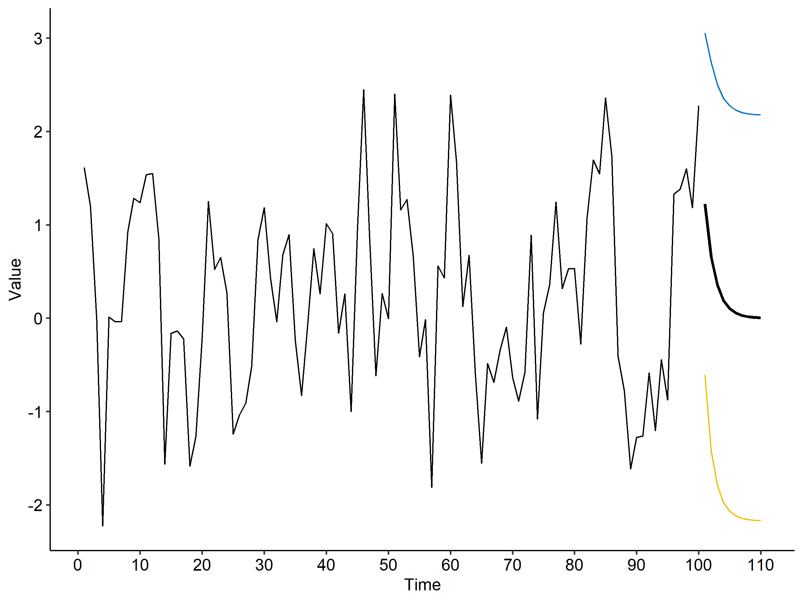
We can also visualize the forecasted values6 and prediction intervals. The bold line shows the predicted values, and the blue and yellow lines are the upper and lower limits of the prediction interval, respectively.
MA
Estimation and forecasting is much simpler in the MA model because the autocorrelation in an MA(q) series disappears after lag $q$. For an MA(1) model:
$$ X_t = \mu + Z_t + \theta Z_{t-1}, $$
Lag 1 forecast
$$ \begin{aligned} X_t(1) &= E(X_{t+1} \mid X_t, X_{t-1}, \cdots, X_1) \\ &= E(\mu + Z_{t+1} + \theta Z_t \mid X_t, X_{t-1}, \cdots, X_1) \\ &= \mu + E(Z_{t+1} \mid X_t, X_{t-1}, \cdots, X_1) + \theta E(Z_t \mid X_t, X_{t-1}, \cdots, X_1) \\ &= \mu + 0 + \theta Z_t = \mu + \theta Z_t \\ \hat{X}_t(1) &= \hat\mu + \hat\theta \hat{Z}_t \end{aligned} $$
The forecasting error is
$$ \begin{aligned} e_t(1) &= X_{t+1} - X_t(1) \\ &= \mu + Z_{t+1} + \theta Z_t - (\mu + \theta Z_t) \\ &= Z_{t+1} \\ Var(e_t(1)) &= \sigma^2 \end{aligned} $$
The $100(1-\alpha)\%$ prediction interval for $X_t(1)$ is thus
$$ \hat\mu + \hat\theta \hat{Z}t \pm Z\frac{\alpha}{2} \cdot \hat\sigma $$
So how do we estimate $\hat{Z}_t$? One way of doing it is
$$ \begin{gathered} X_t = Z_t + \hat\theta Z_{t-1} + \hat\mu \\ Z_t = X_t - \hat\theta Z_{t-1} - \hat\mu \\ Z_{t-1} = X_{t-1} - \hat\theta Z_{t-2} - \hat\mu \\ \vdots \\ Z_2 = X_2 - \hat\theta Z_1 - \hat\mu \\ Z_1 = X_1 - \hat\theta Z_0 - \hat\mu \end{gathered} $$
where $Z_0 = 0$. Now going from bottom up we’d be able to estimate $Z_t$.
Lag 2 forecast
The 2 time ahead forecast is
$$ \begin{aligned} X_t(2) &= E(X_{t+2} \mid X_t, X_{t-1}, \cdots, X_1) \\ &= E(\mu + Z_{t+2} + \theta Z_{t+1} \mid X_t, X_{t-1}, \cdots, X_1) \\ &= \mu \end{aligned} $$
The forecasting error is
$$ \begin{aligned} e_t(2) &= X_{t+2} - X_t(2) = Z_{t+2} + \theta Z_{t+1} \\ Var(e_t(2)) &= Var(Z_{t+2} + \theta Z_{t+1}) \\ &= \sigma^2 + \theta^2 \sigma^2 = (1 + \theta^2)\sigma^2 \end{aligned} $$
Thus the $100(1-\alpha)\%$ prediction interval for $X_t(2)$ is
$$ \hat\mu \pm Z_{\frac{\alpha}{2}} \cdot \sqrt{(1 + \hat\theta^2)\hat\sigma^2} $$
General case
The lag $k$ forecast is
$$ X_t(k) = E(X_{t+k} \mid X_t, X_{t-1}, \cdots, X_1) = \mu \quad (k \geq 2) $$
The forecasting error is
$$ e_t(k) = X_{t+k} - X_t(k) = Z_{t+k} + \theta Z_{t+k-1} $$
and its variance is
$$ Var(e_t(k)) = (1 + \theta^2)\sigma^2 \quad (k \geq 2) $$
which is equal to $Var(X_t)$. Finally, the $k$ time ahead prediction at $t=T$ and its $95\%$ prediction interval is
$$ \hat{X}_T(k) = \hat\mu, \quad \hat\mu \pm 1.96\sqrt{1 + \hat\theta^2}\hat\sigma $$
ARMA(1, 1)
The model is given by
$$ X_t - \mu = \phi(X_{t-1} - \mu) + Z_t + \theta Z_{t-1} $$
The forecasts are
$$ \begin{aligned} X_t(1) &= E(X_{t+1} \mid X_t, X_{t-1}, \cdots, X_1) = \mu(1 - \phi) + \phi X_t + \theta Z_t \\ X_t(2) &= E(X_{t+2} \mid X_t, X_{t-1}, \cdots, X_1) = \mu(1 - \phi) + \phi X_t(1) \\ X_t(k) &= E(X_{t+k} \mid X_t, X_{t-1}, \cdots, X_1) = \mu(1 - \phi) + \phi X_t(k-1) \quad (k \geq 2) \end{aligned} $$
The forecasting error is
$$ E(e_t(k)) = 0, \quad Var(e_t(k)) \approx Var(X_t) \quad \text{ as } k \rightarrow \infty $$
Questions: 1. What does $\hat{Z}_t$ stand for in the prediction intervals? 2. The df in Ljung-Box test is lag $m$ - number of parameters. What if $m$ is smaller than the number?
Follow the principle of parsimony. ↩︎
$l+1$ puts an emphasize on the intercept term in the model. ↩︎
We ignore $\sigma^2$ when counting the number of parameters. ↩︎
The function returns a
ggmultiplotclass object.↩︎1 2 3library(ggfortify) ggtsdiag(x.fit, gof.lag = 20) + ggpubr::theme_pubr()The degrees of freedom in R’s function is wrong. It’s fixed at $m$. ↩︎
The code for plotting the forecasted values.
↩︎1 2 3 4 5 6 7 8 9 10 11 12 13 14 15 16 17dat.x <- enframe(x) %>% select(Time = name, Value = value) dat.x.fore <- enframe(x.fore$pred) %>% select(Time = name, Value = value) %>% mutate(Time = Time + 100, Upper = U, Lower = L) ggplot(dat.x, aes(x = Time, y = Value)) + geom_line() + geom_line(data = dat.x.fore, size = 1) + geom_line(data = dat.x.fore, aes(y = Upper), color = "#0073C2") + geom_line(data = dat.x.fore, aes(y = Lower), color = "#EFC000") + ggpubr::theme_pubr() + scale_x_continuous(breaks=seq(0, 110, 10)) + theme(legend.position = "none")
| Nov 17 | Spectral Analysis | 9 min read |
| Nov 02 | Decomposition and Smoothing Methods | 14 min read |
| Sep 12 | ARMA Model | 8 min read |
| Sep 04 | Moving Average Model | 6 min read |
| Aug 28 | Autoregressive Series | 9 min read |