Introduction
To understand what a time series is, we first introduce the concept of a stochastic process, which is a collection of random variables $\{X_t\}$ indexed by $t$.
Let’s say $N$, the number of accidents in Athens in $[0, T]$, is a Poisson random variable with mean $\mu$. Here $T$ is fixed, and we have
$$ P(N=n) = \frac{e^{-\mu}\mu^n}{n!} $$
A Poisson process is defined as
$$ N_t = \text{# of accidents in Athens in } [0, t] $$
where $t$ varies on a continuous scale.
A time series is a discretized stochastic process, with each one being recorded at a specific time $t$. In general, data obtained from observations collected sequentially over time can be considered as time series data. This is extremely common:
- Business: weekly interest rates, daily closing stock prices, yearly sales figures, etc.
- Meteorology: daily high/low temperatures, annual precipitation indices, hourly wind speeds, etc.
- Biological sciences: electrical activity of the heart at millisecond intervals
Typically, there’s a serial correlation between the observed data which limits our ability to use conventional statistical analysis methods, as our data are not independent anymore. Studying models that incorporate dependence is the key concept in time series analysis. The models are then used to forecast future observations.
Objectives of time series analysis
When we look at a time series, we first look for mean and variance changes over time by setting up a hypothetical probability model to represent the data. We’re also interested in patterns that occur over time (e.g. seasonal components), and serial correlation between observations.
Some objectives of time series analysis include separation of noise from signals, prediction of future values of a series, predicting one series from observations of another, and controlling future values of a series by adjusting parameters.
In time series analysis we apply mathematical and statistical tests to data to quantify and understand the nature of time-varying phenomena, thus gaining physical understanding of the system.
In this course we assume that the data are collected regularly, i.e. regularly spaced time series where the set $T_0$ of times at which observations are made is a discrete set. For example, $\{X_t\}, t = 1, 2, \cdots$.
Mean and covariance
Let $X, Y$ be random variables and $a$, $b$, $c$ and $d$ be constants. The expectation and variance for $X$ have properties:
$$ \begin{gathered} E(aX + b) = a E(X) + b \\ Var(aX + b) = a^2 Var(X) \end{gathered} $$
The covariance term is given by:
$$ \begin{aligned} Cov(aX + b, cY + d) &= Cov(aX, cY) + Cov(aX, d) + Cov(b, cY) + Cov(b, d) \\ &= acCov(X, Y) \end{aligned} $$
Independence indicates zero covariance, but not vice versa.
The variance also has property:
$$ \begin{aligned} Var(aX + bY + c) &= Var(aX + bY) \\ &= Var(aX) + Var(bY) \pm 2ab Cov(X, Y) \\ &= a^2Var(X) + b^2Var(Y) \pm 2abCov(X, Y) \end{aligned} $$
Let $\{X_t\}$ be a time series with $E(X_t^2) < \infty$. The mean function is
$$ \mu_X (t) = E(X_t) = \int xf(x)dx $$
The covariance function is
$$ \gamma_X(t, s) = Cov(X_t, X_s) = E\left[ (X_t - \mu_X(t))(X_s - \mu_X(s)) \right] $$
for all integers $t$ and $s$.
Stationarity
If a time series is strong stationary or strictly stationary, $(X_1, \cdots, X_n)$ and $(X_{1+h}, \cdots, X_{n+h})$ have the same joint distributions for all integers $h$ and $n \geq 1$. If a process is strictly stationary and has finite variance, then the covariance function must depend only on the time lag. An i.i.d. sequence is strictly stationary.
In weak stationarity we don’t have to explicitly deal with the multivariate distributions. Much of the information in these joint distributions can be described in terms of the first- and second-order moments of the joint distributions, i.e. means, variances and covariances. The conditions are:
- $\mu_X(t)$ is independent of $t$, i.e. $\mu_X(t) = \mu$.
- $\gamma_X(t, s) = Cov(X_t, X_s)$ only depends on the time lag $|t - s|$, i.e. $\gamma_X(t, s) = \gamma_X(|t - s|)$. For example, for a stationary series $\gamma(15, 10)$ = $\gamma(0, 5)$ = $\gamma(7, 2)$ etc.
Weak stationarity does not imply strict stationarity, and in this class the term “stationary” always refers to weak stationary unless specifically indicated.
Example 1
Show that $X_t = Z_t + 0.4 Z_{t-1}$ is stationary where $Z_t \overset{i.i.d.}{\sim} N(0, 1)$.
We first show the expected value is constant over time:
$$ \begin{aligned} E(X_t) &= E(Z_t + 0.4 Z_{t-1}) \\ &= E(Z_t) + 0.4 E(Z_{t-1}) = 0 \end{aligned} $$
Then we find the covariance term:
$$ \begin{aligned} \gamma_X(t, s) &= Cov(X_t, X_s) \\ &= Cov(Z_t + 0.4 Z_{t-1}, Z_s + 0.4 Z_{s-1}) \\ &= Cov(Z_t, Z_s) + 0.4 Cov(Z_t, Z_{s-1}) + 0.4 Cov(Z_{t-1}, Z_s) + 0.16 Cov(Z_{t-1}, Z_{s-1}) \end{aligned} $$
Here we have to consider several cases. When $t=s$,
$$ \begin{aligned} \gamma_X(t, s) &= Cov(Z_t, Z_t) + 0.4 Cov(Z_t, Z_{t-1}) + 0.4 Cov(Z_{t-1}, Z_t) + 0.16 Cov(Z_{t-1}, Z_{t-1}) \\ &= Var(Z_t) + 0 + 0 + 0.16 Var(Z_{t-1}) \\ &= 1 + 0.16 = 1.16 \end{aligned} $$
where two of the covariance terms are zero because $Z_t$’s are independent by definition.
When $t=s-1$,
$$ \begin{aligned} \gamma_X(t, s) &= Cov(Z_{s-1}, Z_s) + 0.4 Cov(Z_{s-1}, Z_{s-1}) + 0.4 Cov(Z_{s-2}, Z_s) + 0.16 Cov(Z_{s-2}, Z_{s-1}) \\ &= 0 + 0.4 + 0 + 0 = 0.4 \end{aligned} $$
When $t-1 = s$,
$$ \begin{aligned} \gamma_X(t, s) &= Cov(Z_t, Z_{t-1}) + 0.4 Cov(Z_t, Z_{t-2}) + 0.4 Cov(Z_s, Z_s) + 0.16 Cov(Z_s, Z_{s-1}) \\ &= 0.4 \end{aligned} $$
For all other cases, $\gamma_X(t, s) = 0$ because of the independence. In summary,
$$ \gamma_X(t, s) = \begin{cases} 1.16, & |t-s| = 0 \\ 0.4, & |t-s| = 1 \\ 0, & \text{otherwise} \end{cases} \qquad = \gamma_X(|t-s|) $$
Thus we’ve shown that $X_t$ is stationary.
Example 2
Show that $X_t = X_{t-1} + Z_t$ is nonstationary where $Z_t \overset{i.i.d.}{\sim} N(0, 1)$.
To show nonstationarity we don’t have to go through the entire process above. We only need to show that either the mean is not a constant, or the variance changes over time. Note that
$$ \begin{gathered} X_{t-1} = X_{t-2} + Z_{t-1} \\ X_{t-2} = X_{t-3} + Z_{t-2} \\ X_{t-3} = X_{t-4} + Z_{t-3} \\ \vdots \end{gathered} $$
Since there’s no $Z_t$ term in $X_{t-1}$, the covariance between $X_{t-1}$ and $Z_t$ is 0.
$$ \begin{aligned} Var(X_t) &= Var(X_{t-1} + Z_t) \\ &= Var(X_{t-1}) + Var(Z_t) + 0 \\ &= 1 + Var(X_{t-2} + Z_{t-1}) \\ &= 2 + Var(X_{t-3} + Z_{t-2}) \\ &= t + Var(X_0) \end{aligned} $$
where $X_0$ is the initial point (constant) and the variance is equal to zero. So $Var(X_t) = t$ and it changes over time, which means $X_t$ is nonstationary.
Autocovariance and autocorrelation
The autocovariance function (ACVF) and autocorrelation function (ACF) are key tools for identifying stationarity. Let $\{X_t\}$ be a stationary time series, the autocovariance function at lag $k$ is given by
$$ \gamma_X(k) = Cov(X_t, X_{t-k}), k \in \mathbb{Z} $$
Some properties are:
- $Var(X_t) = \gamma_X(0)$, which implies that the variance doesn’t change over time.
- $\gamma_X(k) = \gamma_X(-k)$, the function is symmetric and the difference stays the same.
- $|\gamma_X(k)| \leq \gamma_X(0)$. None of the covariance terms can be greater than the variance.
A real-valued function defined on the integers is the autocovariance function of a stationary time series if and only if it’s even and nonnegative definite (or semi-positive definite), i.e.
$$ \sum_{i=1}^T \sum_{j=1}^T a_i \gamma(i-j)a_j \geq 0 $$
for all positive integers $T$ and real vectors $\boldsymbol{a} = (a_1, \cdots, a_T)^\prime$.
The autocorrelation function is the correlation between $X_t$ and each of the previous values $X_{t-1}$, $X_{t-2}$, … At lag $k$, it is
$$ \rho_X(k) = Corr(X_t, X_{t-k}) = \frac{Cov(X_t, X_{t-k})}{\sqrt{Var(X) Var(X_{t-k})}} = \frac{\gamma_X(k)}{\gamma_X(0)}, k \in \mathbb{Z} $$
By definition we have $\rho_X(0) = 1$ and $\rho_X(k) = \rho_X(-k)$.
Sample version
In practical problems we don’t start with a model, but with observed data (a sample). Let $\{X_t\}$ be observations of a time series. To estimate the autocovariance function, the sample autocovariance function is given by
$$ \hat\gamma_X(k) = \frac{1}{T}\sum_{t=1}^{T-k}(X_t - \bar{X})(X_{t+k} - \bar{X}) $$
where $\bar{X} = \frac{1}{T}\sum_{t=1}^T X_t$ is the sample mean.
The sample autocorrelation function is
$$ \hat\rho_X(k) = \frac{\hat\gamma_X(k)}{\hat\gamma_X(0)} = \frac{\sum_{t=1}^{T-k}(X_t - \bar{X})(X_{t+k} - \bar{X})}{\sum_{t=1}^T (X_t - \bar{X})^2} $$
PACF and SPACF
Two other useful tools to identify autocorrelation are the partial ACF (PACF) and the sample PACF. To understand where these came from, recall that in simple linear regression we have
$$ Y = \beta_0 + \beta_1 X + \epsilon, $$
where we often assume that $\epsilon \sim N(0, \sigma^2)$ and the independence of $X$ and $\epsilon$. We can drop the intercept term if $X$ and $Y$ are standardized, and the covariance between $X$ and $Y$ would be
$$ \begin{aligned} Cov(X, Y) &= Cov(X, \beta_1 X + \epsilon) \\ &= \beta_1 Cov(X, X) + Cov(X, \epsilon) \\ &= \beta_1 \end{aligned} $$
The correlation between $X$ and $Y$ would be
$$ Corr(X, Y) = \frac{Cov(X, Y)}{\sqrt{Var(X) Var(Y)}} = \beta_1 $$
So the slope in SLR is the correlation if $X$ and $Y$ are standardized. If they are not standardized,
$$ Corr(X, Y) \propto \beta_1 $$
This is why $H_0: \beta_1 = 0$ and $H_0: \rho = 0$ are the same in SLR.
In multiple linear regression, again assuming the variables are standardized, we have
$$ Y = \beta_1 X_1 + \cdots + \beta_p X_p + \epsilon $$
Here $\beta_j \neq Corr(X_j, y)$ or otherwise we can just run multiple correlation instead of regression. The partial correlation is actually
$$ \beta_j = Corr(X_j, Y \mid X_1, \cdots, X_{j-1}, X_{j+1}, \cdots, X_p) $$
To understand this, if we just look at the correlation between one’s math score and height, the value might be very large. However, we’ve missed a hidden variable of one’s age, and once we include that,
$$ Corr(\text{Height, Score} \mid \text{Age/Grade}) \approx 0 $$
The partial ACF is the correlation between two timepoints, given the values of the time series in between:
$$ \phi_{kk} = Corr(X_t, X_{t-k} \mid X_{t-1}, X_{t-2}, \cdots, X_{t-k+1}) $$
When $k=1$, $\phi_{11} = Corr(X_t, X_{t-1}) = \rho_X(1)$ because there’s no time series values between $X_t$ and $X_{t-1}$.
The sample PACF, $\hat\phi_{kk}$, is found by the OLS estimate of $\phi_{kk}$ in the following:
$$ X_t = \phi_{k1} X_{t-1} + \phi_{k2}X_{t-2} + \cdots + \phi_{kk}X_{t-k} + Z_t $$
This explains why we need two indices: say $k=3$, we’re only interested in the third coefficient in the $k=3$ case.
Basic models
In the following examples, we shall talk about two very common time series models utilizing the concepts we’ve introduced above.
White noise
The simplest kind of time series is a collection of independent and identically distributed random variables with mean zero and constant variance. $Z_t$ is white noise if
$$ E(Z_t) = 0 \text{ and } \gamma_Z(k) = \sigma^2 I(k=0) $$
where $I(k=0)$ is an indicator function. This is denoted $\{X_t\} \sim WN(0, \sigma^2)$.
Most often, the probability distribution is assumed to be normal, then this is written as $Z_t \sim N(0, \sigma^2)$, meaning that each $Z_t$ has a normal distribution with mean 0 and constant variance $\sigma^2$. $Z_1, \cdots, Z_T$ are independent of each other.
For a WN process, two approximate standard errors (95.4%) of the sample ACF are $\pm\frac{2}{\sqrt{n}}$1. If all $\hat\rho_X(k)$ are within the limits, the process could be considered as WN. We can show this in R2 using simulated data where $n=100$ and $\sigma^2 = 1$.
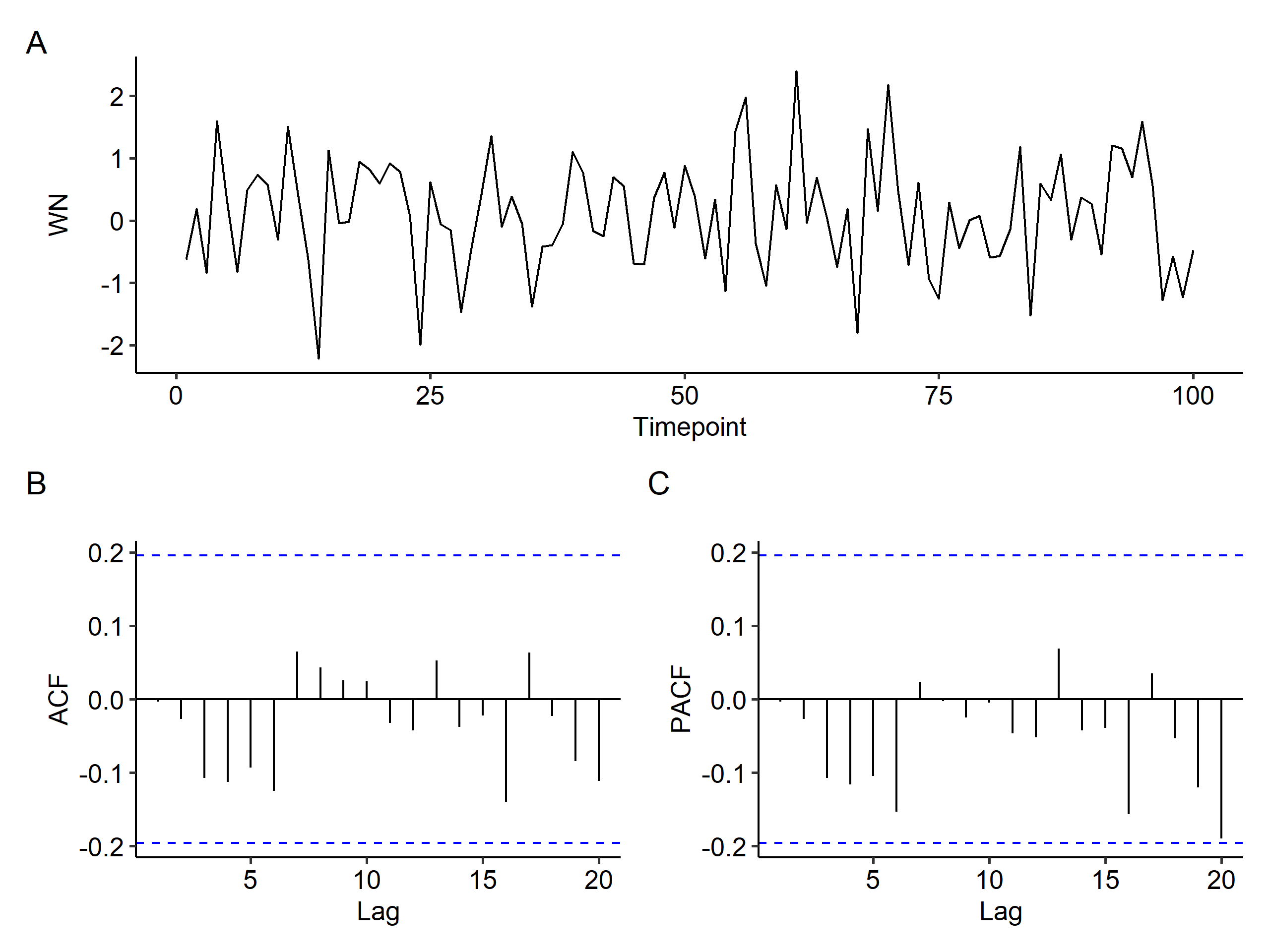
As shown above, all ACF fall within $\pm 0.2$. The hypothesis $H_0: \rho_X(k) = 0$ can be rejected at the usual significance levels, in our case $0.05$.
Random walk
$\{X_t\}$ is a random walk if it can be represented as
$$ X_t = X_{t-1} + Z_t $$
where $Z_t$ is $WN(0, \sigma^2)$. There’s no particular pattern, and we’re just cumulatively summing i.i.d. (standard normal) random variables. In a random walk, $Z_t$ is the size of the steps, $X_t$ is the position of the random walker at time $t$, $E(X_t) = 0$, and $Var(X_t) = t\sigma^2$, meaning that it’s nonstationary.
Movement of common stock prices, position of small particles suspended in a fluid are examples of random walks. Of course we can generate simulated data3 and study its behavior:
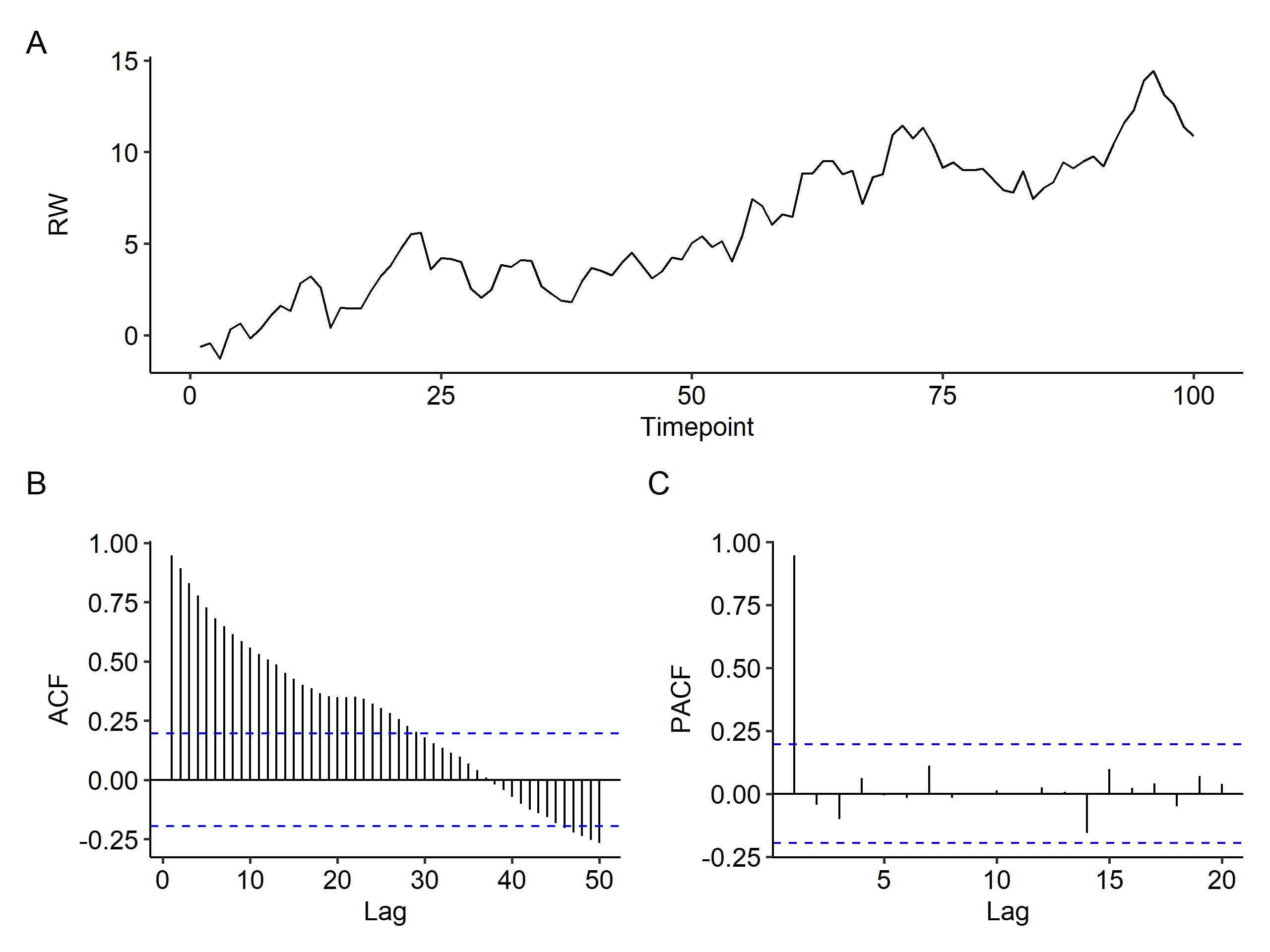
The trend in the ACF is very typical for RW data. It starts from $\rho(0) = 1$, then slowly decreases because each value depends on the previous value. However, the PACF doesn’t show such trends. If we see such patterns in a samples ACF and PACF, the RW is a potential model (but not the only one!).
This is found by $1.96 \times \frac{\sigma}{\sqrt{n}}$. $\sigma$ is set to 1 because the data are standardized. ↩︎
The R code for simulating white noise and plotting.
↩︎1 2 3 4 5 6 7 8 9 10 11 12 13 14 15 16 17 18 19 20 21 22 23 24 25 26 27 28library(tidyverse) library(forecast) library(patchwork) theme_set(ggpubr::theme_pubr()) plot_time_series <- function(x, x_type = "WN", lag.max = NULL) { x_acf <- acf(x, lag.max = lag.max, plot = F) x_pacf <- pacf(x, plot = F) dat <- tibble( Timepoint = seq(length(x)), x = x ) p1 <- ggplot(dat, aes(Timepoint, x)) + geom_line() + labs(y = x_type) p2 <- autoplot(x_acf) + ggtitle("") p3 <- autoplot(x_pacf) + ggtitle("") p1 / (p2 | p3) + plot_annotation(tag_levels = 'A') } set.seed(1) wn_val <- rnorm(n = 100, mean = 0, sd = 1) plot_time_series(wn_val, x_type = "WN")The code for simulating random walk data. The max lag is increased to show the trend. Sometimes we extend this to show seasonal trends.
↩︎1 2 3set.seed(1) x <- gen_random_walk(100, 0, 1) plot_time_series(x, x_type = "RW", lag.max = 50)
| Nov 23 | Conditional Heteroscedastic Models | 15 min read |
| Nov 17 | Spectral Analysis | 9 min read |
| Nov 02 | Decomposition and Smoothing Methods | 14 min read |
| Sep 14 | Model Fitting and Forecasting | 15 min read |
| Sep 12 | ARMA Model | 8 min read |