Mean Trend
Previously we assumed time series to be stationary in order to use the statistical methods discussed. Unfortunately, more real-world data are not stationary. In this chapter, we will focus on nonstationary time series, starting with processes whose mean change over time.
There could be two types of nonstationary time series, the first one being the mean changing over time. The mean could change with a seasonal pattern, or it could show an overall trend of increase/decrease. Not all kinds of changes can be dealt with, and we’ll discuss the limitations later.
We start with the mean trend where we decompose a time series into two parts:
$$ X_t = \mu_t + W_t $$
Here $\mu_t$ is a trend over time and $W_t$ is a stationary time series with mean 0. The mean $\mu_t$ can be viewed as deterministic or stochastic. A deterministic trend is valid for a given time period and in the future, meaning that we believe the trend we’re seeing in the data continues in the future. A stochastic trend is not deterministic, but shows some overall trends over a long time period. A random walk is an example that contains a stochastic trend.
Stochastic trends are frequently used in finance, and is more challenging in terms of modeling and prediction. In this course we mostly focus on deterministic trends as it’s easier to deal with. The key difference between the two is whether the trend is random or not.
Below is one example of a nonstationary series from the TSA R library1. The mean is obviously not constant over time. It was sort of stable from 1986 to 1995, but somewhere around 1999 it went up.
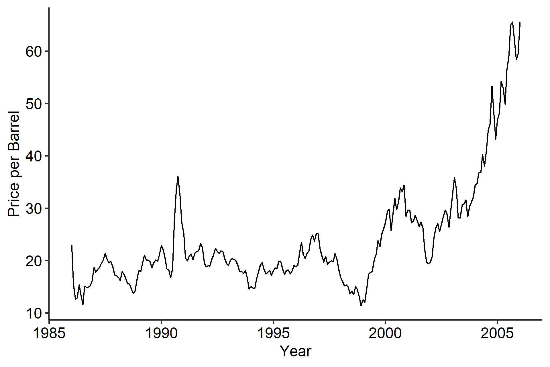
A question here is will this increasing trend continue in the future? Probably not, as at some point we’d expect it to go down again, so we should think of it as a stochastic trend.
Another example is the explosive AR(1). Previously we showed that the stationary condition for an AR(1) model is $|\phi| < 1$. But when $|\phi| > 1$, for example
$$ X_t = 3X_{t-1} + Z_t = Z_t + 3Z_{t-1} + 3^2 Z_{t-2} + \cdots + 3^{t-1}Z_1 + 3^t X_0, $$
the impact of data in the past exponentially increases2. It’s called explosive because $X_t$ more and more depends on the past data.
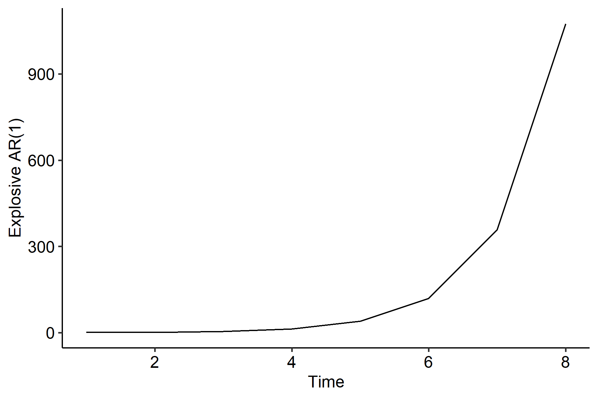
We’ll soon learn that the trend in the oil price example could be handled, whereas the explosive AR(1) case could not.
So how do we remove a deterministic trend (or some part of a stochastic trend) and make a series stationary? There are two approaches: detrending and differencing.
Detrending
In detrending we fit a trend using parametric regression or nonparametric smoothing, and subtract it from the original series. This method is only valid when we have a deterministic trend. For example,
$$ \begin{gathered} X_t = \beta_0 + \beta_1 t + D_t \\ \hat{D}_t = X_t - \hat\beta_0 - \hat\beta_1 t \end{gathered} $$
Here we decomposed the time series $X_t$ into a linear part $\beta_0 + \beta_1$ and a stationary part. Once we have the estimated $\hat\beta_0$ and $\hat\beta_1$, the residuals $\hat{D}_t$ will be stationary and we can apply an ARMA model. The regression part is very flexible, and we can fit whatever model that’s necessary to remove the trend.
This method is popular, but it comes with several problems. First, the trend has to be deterministic. Second, when the trend is more complicated than a simple linear regression, we may introduce unnecessary bias. nonparametric smoothing is applied to reduce this bias.
Differencing
Often differencing is used to account for nonstationarity that occurs in the form of trend and/or seasonality. Differencing can deal with deterministic trends and some types of stochastic trends.
Differencing is performed by subtracting the previous observation from the current observation. The first order differencing is
$$ \nabla X_t = X_t - X_{t-1} = (1-B)X_t $$
where $B$ is the backshift operator. $(1-B)$ can be thought of as a linear filter since the linear trend is being filtered out of the time series. Going back to the example of $X_t = \beta_0 + \beta_1 t + D_t$, the first order differencing would be
$$ X_t - X_{t-1} = \beta_0 + \beta_1 t + D_t - \beta_0 - \beta_1 (t-1) - D_{t-1} = \beta_1 + D_t - D_{t-1}, $$
which is a linear combination of stationary series and is thus stationary.
Similarly, the second order differencing of a time series is
$$ \begin{aligned} \nabla^2 X_t &= \nabla(\nabla X_t) \\ &= \nabla (X_t - X_{t-1}) \\ &= (X_t - X_{t-1}) - (X_{t-1} - X_{t-2}) \\ &= X_t - 2X_{t-1} + X_{t-2} \\ &= (1 - 2B + B^2)X_t \\&= (1-B)^2 X_t \end{aligned} $$
Second order differences will help remove quadratic trends, which can be shown similarly. If we repeat the differencing $d$ times,
$$ \nabla^d = (1-B)^d $$
where $d$ is called the order of differencing. In most cases $d=1$ is enough, and sometimes $d=2$. Differencing should be considered when the ACF of a time series slowly decreases.
Simulation in R
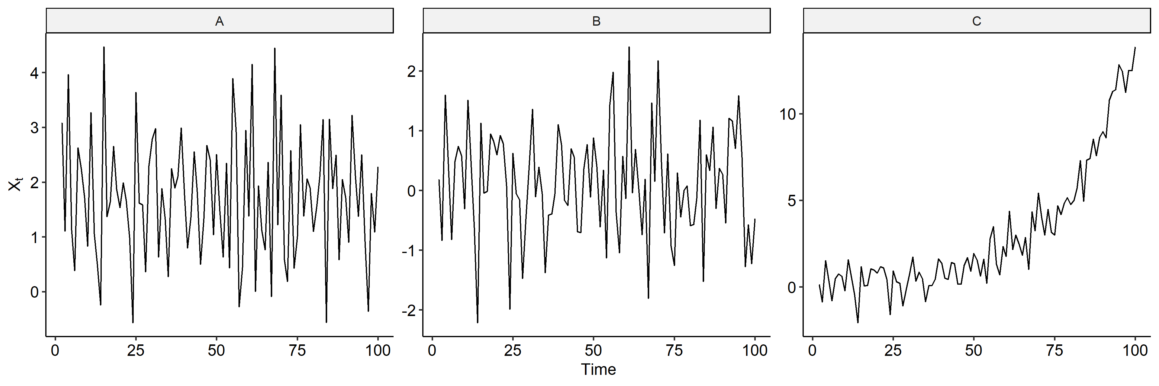
We are going to simulate three time series and try to remove the mean trend using detrending and differencing:
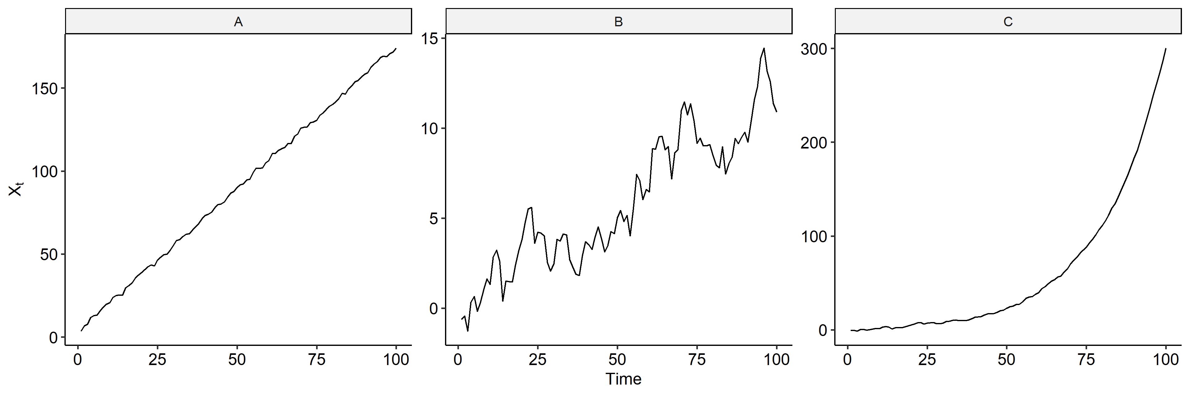
$$ \begin{aligned} A&: X_t = 3 + 1.2t + 0.3 X_{t-1} + Z_t \\ B&: X_t = X_{t-1} + Z_t \\ C&: X_t = 1.05 X_{t-1} + Z_t \end{aligned} $$
where $Z_t$ is $WN(0, 1^2)$. We can see that model A is a linear model plus an AR(1) model, model B is a random walk, and model C is an AR(1) model with $|\phi| > 1$.
| |
We can plot the series to see how they change over time3. There’s a clear linear trend in model A. Model B looks like it’s increasing but that’s just the characteristics of a random walk. Model C is exponentially increasing. Note the scales on the y-axis are different.
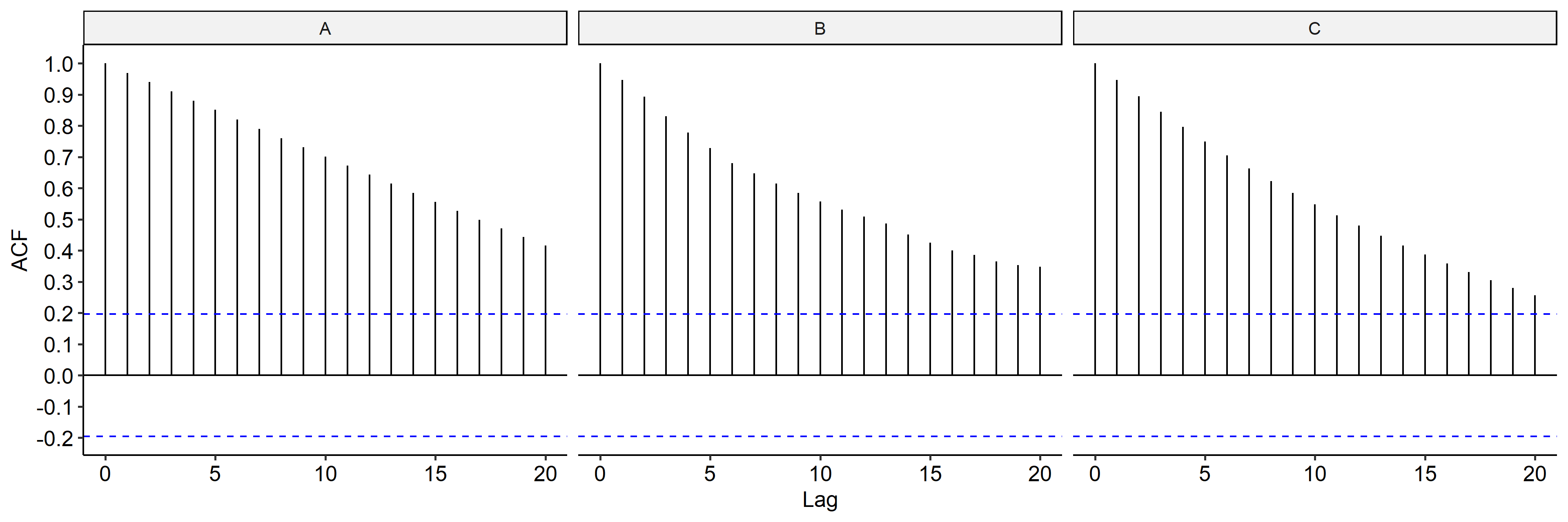
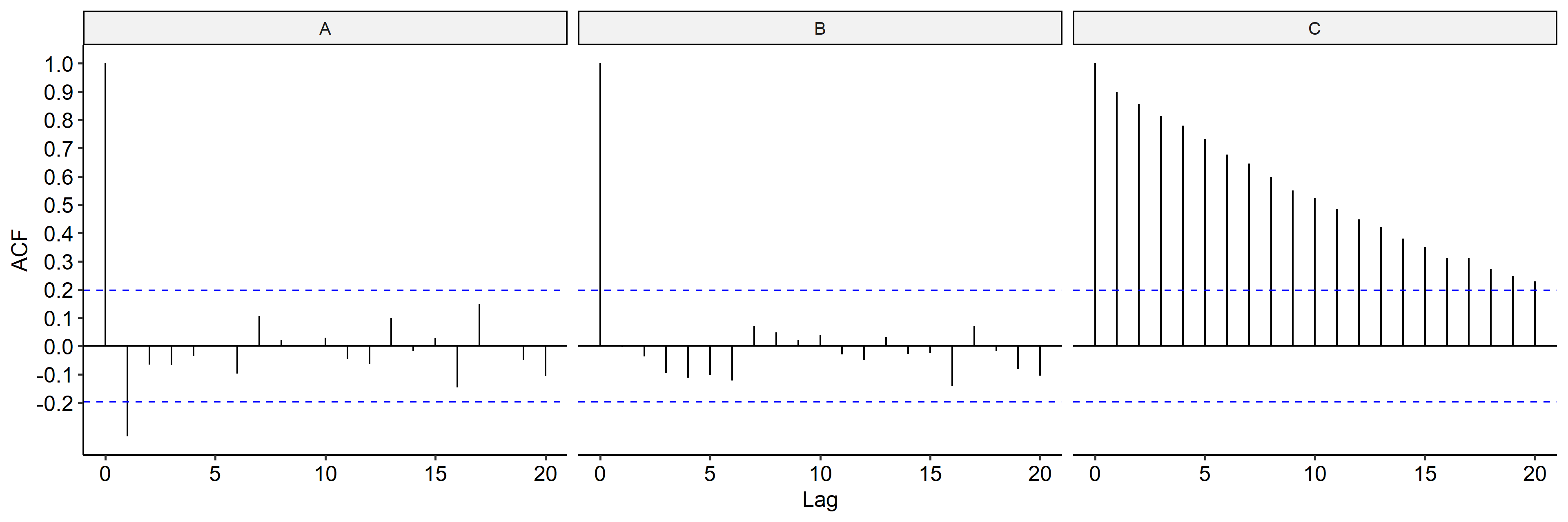
Next we check the ACF for the three models4. In all three cases the ACFs seem to be slowly decreasing, indicating differencing might be applied to remove the trend.
Differencing
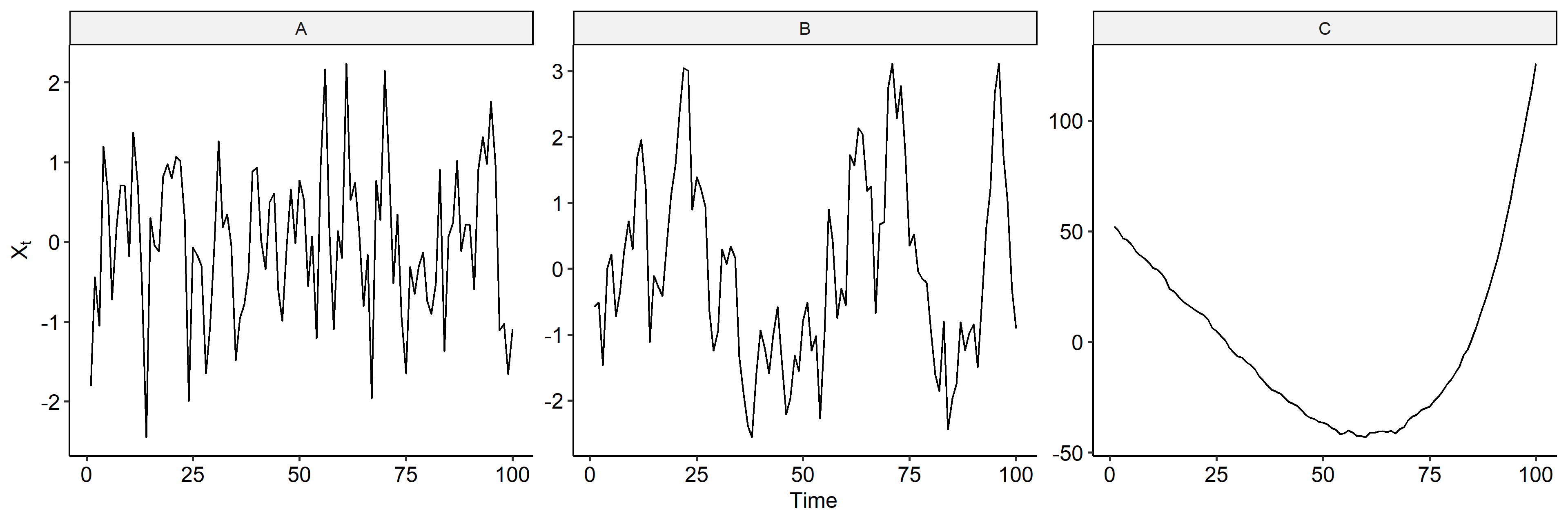
Now we may calculated the lagged differences in R using the diff function. After first order differencing5, model A looks like a stationary series and we don’t see the linear trend. Model B is also somewhat stationary, but model C still shows an increasing mean trend.
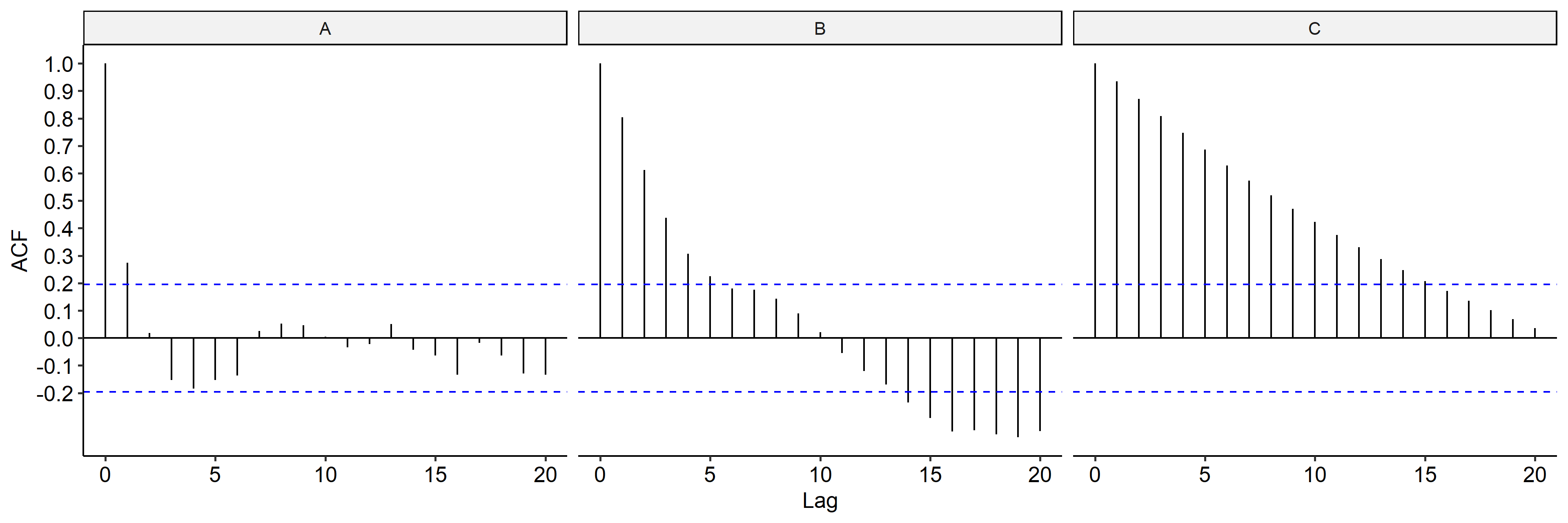
We can also check the ACF of the differenced series to confirm our conclusions6. Indeed, the ACF of model A is cut off after lag 1; everything is within the bands for model B; ACF for model C didn’t change much.
Detrending
We will use model A as an example. Recall that the data generating model is
$$ X_t = 3 + 1.2t + 0.3 X_{t-1} + Z_t $$
And if we fit a simple linear regression model in R:
| |
The estimated parameters for the linear trend are $\hat\mu = 3.666$ and $\hat{t} = 1.715$. We can extract the detrended series using fit$residuals. If we apply the same method on models B and C, below are the detrended time series.
It looks like in model A detrending worked well. Model B still doesn’t look stationary after detrending, and neither does mode C. As confirmed in the ACF plot, models B and C still show autocorrelation after detrending.
More on Differencing
Differencing is more flexible than detrending, and works better in many cases. Differencing makes sense when a trend slowly changes over time. Consider the following time series model:
$$ X_t = \mu_t + W_t $$
where $\mu_t$ is the mean that slowly changes over time, and $W_t$ is a stationary series with mean zero. We consider several cases for $\mu_t$, and discuss which types of trends could be removed through differencing.
Case I
$\mu_t$ can be considered as a constant over two time points, i.e. it changes very slowly. Then we can estimate the mean by
$$ \hat\mu_t = \frac{1}{2} (X_t + X_{t-1}) $$
Therefore if we subtract the mean from the original time series,
$$ \begin{aligned} X_t - \hat\mu_t &= X_t - \frac{1}{2} (X_t + X_{t-1}) \\ &= \frac{1}{2} (X_t - X_{t-1}) \\ &= \frac{1}{2}\nabla X_t \end{aligned} $$
which is a constant times the differenced time series. If we take the first order differencing of $X_t$, the resulting time series is $W_t$, a stationary series.
Case II
If $\mu_t$ follows a random walk (stochastic trend),
$$ \mu_t = \mu_{t-1} + e_t, \quad e_t \overset{i.i.d.}{\sim} N(0, \sigma_e^2) $$
where $e_t$ is independent of $W_t = Z_t \overset{i.i.d.}{\sim} N(0, \sigma^2)$7. Then if we apply first order differencing,
$$ \begin{aligned} \nabla X_t &= X_t - X_{t-1} \\ &= \mu_t + W_t - \mu_{t-1} - W_{t-1} \\ &= \mu_t - \mu_{t-1} + Z_t - Z_{t-1} \\ &= e_t + Z_t - Z_{t-1} \end{aligned} $$
is a linear combination of normal random variables, thus an MA(1) model and is stationary. We can show that there’s a spike at lag 1 for the ACF of $X_t$, and all the other ACFs are zero:
$$ \rho_X(1) = -\frac{1}{2 + \sigma_e^2 / \sigma^2} $$
TODO: proof
Case III
This is somewhat a generalization of case I. If $\mu_t$ is locally linear over three time points,
$$ \hat\mu_t = \frac{1}{3}(X_{t+1} + X_t + X_{t-1}) $$
When we subtract the mean from the series,
$$ \begin{aligned} X_t - \hat\mu_t &= X_t - \frac{1}{3}(X_{t+1} + X_t + X_{t-1}) \\ &= -\frac{1}{3}(X_{t+1} - 2X_t + X_{t-1}) \\ &= -\frac{1}{3}\nabla^2 X_{t+1} \end{aligned} $$
So we have the second order differencing
$$ \nabla^2 X_t = -3(X_t - \hat\mu_t) $$
to be stationary. Compared to case I, the mean is slightly more irregularly changing and we could have a overall quadratic trend.
Case IV
This is a more advanced version of case II. Let
$$ X_t = \mu_t + Z_t, \quad \mu_t = \mu_{t-1} + W_t, \quad W_t = W_{t-1} + e_t $$
where $e_t \sim N(0, \sigma_e^2)$ and $Z_t \overset{i.i.d.}{\sim} N(0, \sigma^2)$. The mean trend is stochastic with two layers – a random walk plus the previous value. We need a second order differencing to remove this trend:
$$ \begin{aligned} \nabla^2 X_t &= \nabla(\nabla X_t) = \nabla(X_t - X_{t-1}) \\ &= \nabla(\mu_t + Z_t - \mu_{t-1} - Z_{t-1}) \\ &= \nabla(W_t + Z_t - Z_{t-1}) \\ &= (W_t + Z_t - Z_{t-1}) - (W_{t-1} + Z_{t-1} - Z_{t-2}) \\ &= e_t + Z_t - 2Z_{t-1} + Z_{t-2} \end{aligned} $$
which is a stationary MA(2) process.
Install the
TSApackage to get the dataset.↩︎1 2 3 4 5 6 7 8 9 10 11 12 13library(tidyverse) library(TSA) data("oil.price") tibble( Timepoint = time(oil.price), x = oil.price ) %>% ggplot(aes(Timepoint, x)) + geom_line() + labs(x = "Year", y = "Price per Barrel") + ggpubr::theme_pubr()When $|\phi| = 1$, we have a random walk. ↩︎
R code for plotting the time series.
↩︎1 2 3 4 5 6 7 8 9 10tibble( Timepoint = seq(n), A = x1, B = x2, C = x3 ) %>% pivot_longer(names_to = "Series", values_to = "Value", -Timepoint) %>% ggplot(aes(Timepoint, Value)) + geom_line() + facet_wrap(~ Series, nrow = 1, scales = "free_y") + labs(x = "Time", y = expression(X[t])) + ggpubr::theme_pubr()R code for calculating the ACF. The dashed blue lines represent an approximate 95% confidence interval for a white noise. ACF falling within the lines indicate no serual correlation.
↩︎1 2 3 4 5 6 7 8 9 10 11 12 13 14 15 16 17 18 19ci <- qnorm((1 + 0.95) / 2) / sqrt(n) # 95% CI tibble( Lag = seq(20), A = acf(x1, plot = F, lag.max = 20)$acf, B = acf(x2, plot = F, lag.max = 20)$acf, C = acf(x3, plot = F, lag.max = 20)$acf, ) %>% mutate_all(as.numeric) %>% pivot_longer(names_to = "Series", values_to = "Value", -Lag) %>% ggplot(aes(Lag, Value)) + geom_segment(aes(x = Lag, xend = Lag, y = 0, yend = Value)) + geom_hline(yintercept = 0) + geom_hline(yintercept = ci, color = "blue", linetype = "dashed") + geom_hline(yintercept = -ci, color = "blue", linetype = "dashed") + scale_y_continuous(breaks = seq(-0.2, 1, 0.1)) + facet_wrap(~ Series, nrow = 1) + labs(x = "Lag", y = "ACF") + ggpubr::theme_pubr()Calculating the lagged differences using
dplyr::lag().↩︎1 2 3 4 5 6 7 8 9 10 11 12 13 14tibble( Timepoint = seq(n), A = x1, B = x2, C = x3 ) %>% mutate(A = A - lag(A), B = B - lag(B), C = C - lag(C)) %>% drop_na() %>% pivot_longer(names_to = "Series", values_to = "Value", -Timepoint) %>% ggplot(aes(Timepoint, Value)) + geom_line() + facet_wrap(~ Series, nrow = 1, scales = "free_y") + labs(x = "Time", y = expression(X[t])) + ggpubr::theme_pubr()R code for preparing the data frame for plotting.
↩︎1 2 3 4 5 6 7 8ci <- qnorm((1 + 0.95) / 2) / sqrt(n - 1) # 95% CI tibble( Lag = seq(0, 20), A = acf(diff(x1, lag = 1), plot = F, lag.max = 20, drop.lag.0 = F)$acf, B = acf(diff(x2, lag = 1), plot = F, lag.max = 20, drop.lag.0 = F)$acf, C = acf(diff(x3, lag = 1), plot = F, lag.max = 20, drop.lag.0 = F)$acf, )$W_t$ can be any stationary process. Here we’re assuming it’s $Z_t$ for simplicity of calculation. ↩︎
| Nov 17 | Spectral Analysis | 9 min read |
| Nov 02 | Decomposition and Smoothing Methods | 14 min read |
| Oct 13 | Seasonal Time Series | 17 min read |
| Oct 09 | Variability of Nonstationary Time Series | 13 min read |
| Oct 05 | ARIMA Models | 9 min read |
 Yi's Knowledge Base