Autoregressive Series

In this chapter, we introduce some of the key properties of an important class of time series known as ARMA (autoregressive moving average) series.
Autoregressive series
Let’s consider a class of time series known as autoregressive (AR) series. The concept of autoregression related past observations of the series to current/future observations of the series using a regression-type model. We’ll simulate 100 values from the following AR(1) model using R1:
$$ X_t = 0.7 X_{t-1} + Z_t, $$
where $Z_t$ values are generated from the standard normal distribution. This is an AR model of order 1 because the current value depends on the value before that, called the lag 1 value. The coefficient $0.7$ tells us how strongly the time series depends on the previous value.
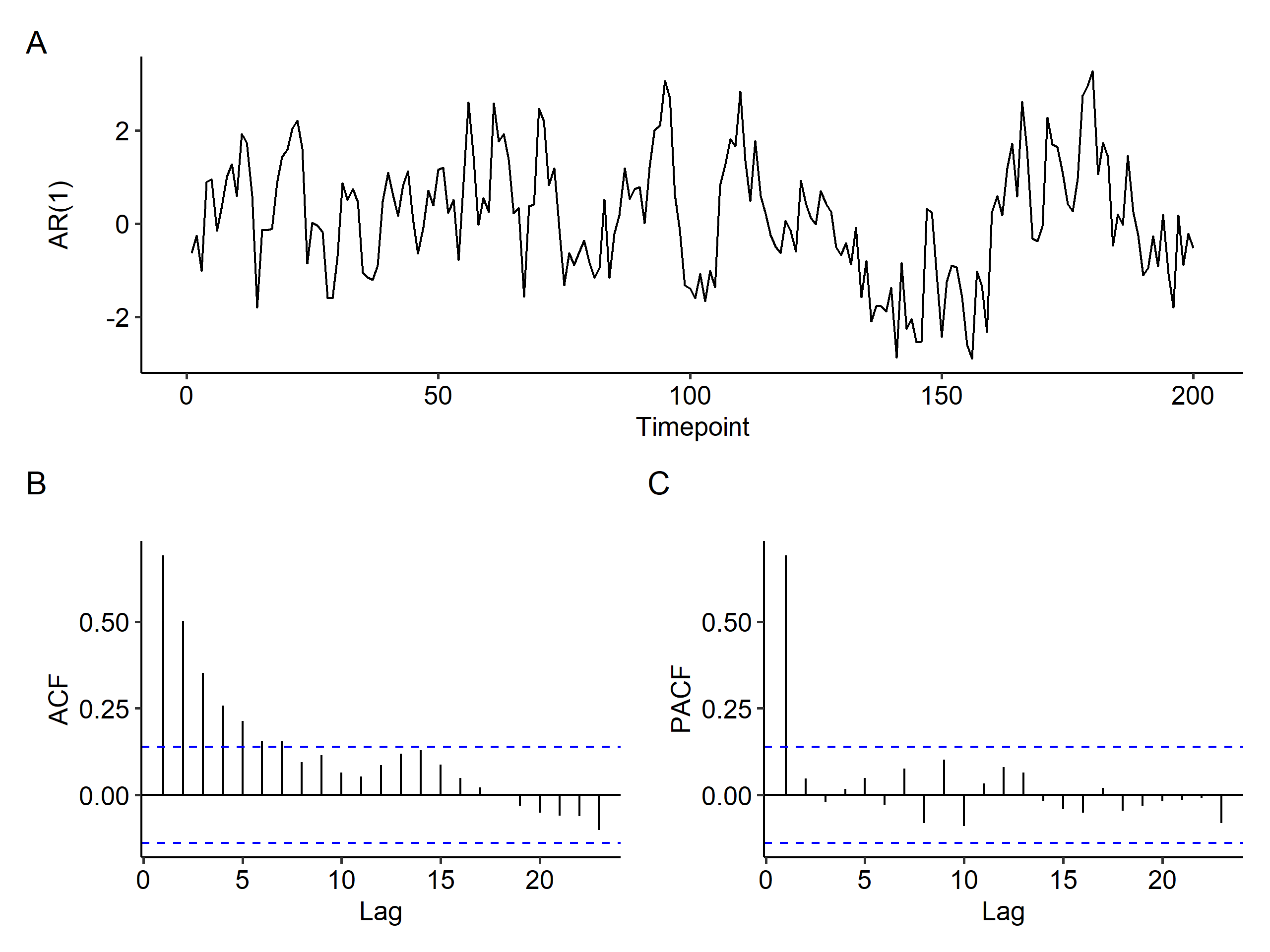
In the time series plot, focusing on timepoint 100 and onwards2, notice how the correlation between adjacent values is high, i.e. neighboring values are close and not jumping around. This is not surprising as we generated the data by setting $X_t$ to be approximately $0.7 X_{t-1}$.
Also, there seems to be a trend of going up and down, and infrequently crossing the theoretical mean of zero (unlike white noise). This trend is due to the strong autocorrelation of neighboring values of the series.
The ACF plot gives the correlations between $X_t$ and $X_{t-1}$, $X_t$ and $X_{t-2}$ etc. Note how the correlation values decrease as the lag increases. Unlike the random walk, this is an exponential decay - the ACF declines very rapidly after some lags and essentially taper off to zero. Exponentially declining autocorrelations is a characteristic of autoregressive series.
The PACF spikes at lag 1 and is essentially zero for other lags. For example, $\phi_{22} \approx 0$, but $\rho_X(2)$ is still large. This could suggest that $X_t$ only depends on $X_{t-1}$. In practice, the interpretation of sample ACF and PACF is not always as clear-cut.
Autoregressive model of order 1
The AR(1) model is:
$$ X_t = \delta + \phi X_{t-1} + Z_t $$
where $|\phi| <1$ (for stationarity) is an autoregressive coefficient, and $Z_t \overset{i.i.d.}{\sim} N(0, \sigma^2)$ is WN which is independent of $X_{t-1}, X_{t-2}, \cdots, X_1$.
Mean
The mean is given by
$$ \begin{gathered} E(X_t) = E(\delta + \phi X_{t-1} + Z_t) = \delta + \phi E(X_{t-1}) + E(Z_t) \\ \mu = \delta + \phi\mu \\ E(X_t) = \mu = \frac{\delta}{1 - \phi} \end{gathered} $$
From this we can easily see that when $\delta = 0$, the mean is also 0.
An alternative expression for AR(1) is
$$ X_t - \mu = \phi(X_{t-1} - \mu) + Z_t $$
This is the format R uses. The expectation is $E(X_t) = \mu$ because
$$ X_t = \underbrace{\mu - \phi\mu}_{\delta} + \phi X_{t-1} + Z_t $$
Variance
For variance and the ACF, we may set $\delta = 0$ without losing any generalizability.
$$ \begin{aligned} Var(X_t) &= Var(\phi X_{t-1} + Z_t) \\ &=Var(\phi X_{t-1}) + Var(Z_t) + \underbrace{2Cov(\phi X_{t-1}, Z_t)}_{=0} \\ &= \phi^2 Var(X_{t-1}) + \sigma^2 \end{aligned} $$
Since $X_t$ is stationary, $Var(X_{t-1}) = Var(X_t)$. So,
$$ Var(X_t) = \frac{\sigma^2}{1 - \phi^2} = \gamma_X(0) $$
We can also validate that the variance is always non-negative because $|\phi| < 1$. In R, we can use the arima.sim function to simulate an ARMA process.
Autocovariance and autocorrelation
$$ \begin{aligned} \gamma_X(1) &= Cov(X_t, X_{t-1}) = Cov(\phi X_{t-1} + Z_t, X_{t-1}) \\ &= \phi Cov(X_{t-1}, X_{t-1}) + Cov(Z_t, X_{t-1}) \\ &= \phi Var(X_{t-1}) \\ &= \phi \gamma_X(0) = \phi \frac{\sigma^2}{1 - \phi^2} \end{aligned} $$
From here we can find the autocorrelation with lag 1:
$$ \rho_X(1) = \frac{\gamma_X(1)}{\gamma_X(0)} = \phi $$
Recall that in the figure, the first lag in the ACF plot is about 0.7.
Next we find the autocovariance with lag 2:
$$ \begin{aligned} \gamma_X(2) &= Cov(X_t, X_{t-2}) \\ &= Cov(\phi X_{t-1} + Z_t, X_{t-2}) \\ &= \phi Cov(X_{t-1}, X_{t-2}) + Cov(Z_t, X_{t-2}) \\ &= \phi \gamma_X(1) = \phi^2 \frac{\sigma^2}{1 - \phi^2} \end{aligned} $$
Now $\rho_X(2)$ can be found:
$$ \rho_X(2) = \frac{\gamma_X(2)}{\gamma_X(0)} = \phi^2 $$
To generalize this, for $k \geq 1$, the autocovariance function is
$$ \begin{aligned} \gamma_X(k) &= Cov(X_t, X_{t-k}) \\ &= Cov(\phi X_{t-1} + Z_t, X_{t-k}) \\ &= \phi Cov(X_{t-1}, X_{t-k}) + Cov(\underbrace{Z_t, X_{t-k}}_{k \geq 1 \Rightarrow \text{indep.}}) \\ &= \phi \gamma_X(k-1) \\ &= \phi^2 \gamma_X(k-2) \\ &= \cdots = \phi^k \gamma_X(0) = \phi^k \cdot \frac{\sigma^2}{1 - \phi^2} \end{aligned} $$
The autocorrelation function is
$$ \rho_X(k) = \frac{\gamma_X(k)}{\gamma_X(0)} = \phi^k $$
We can see that $\rho_X(k)$ is an exponential function, and since $|\phi| < 1$, it exponentially decreases to 0 as the lag increases.
When $\phi$ is large (close to 1), the decay is faster. In R, we can use the ARMAacf function to compute the theoretical ACF for an ARMA process. The same function can be used to find the PACF.
Partial autocorrelation
Theoretically, The PACF is
$$ \phi_{00} = 1,\quad \phi_{11} = \phi = \rho(1), \quad \phi_{kk} = 0 \text{ for } k > 1 $$
The PACF of AR(1) cuts off after lag 1.
Autoregressive model of order $p$
The generalized model is:
$$ X_t = \delta + \phi X_{t-1} + \phi_2 X_{t-2} + \cdots + \phi_p X_{t-p} + Z_t $$
where $Z_t$ is $WN(0, \sigma^2)$.
Expected value
Calculating the expectation for $AR(p)$ is not difficult. Assuming $AR(p)$ is stationary,
$$ \begin{gathered} E(X_t) = \delta + \phi_1 E(X_{t-1}) + \phi_2 E(X_{t-2}) + \cdots + \phi_p E(X_{t-p}) + E(Z_t) \\ \mu (1 - \phi_1 - \phi_2 - \cdots - \phi_p) = \delta \\ \mu = \frac{\delta}{1 - \phi_1 - \phi_2 - \cdots - \phi_p} \end{gathered} $$
The alternative expression in R is:
$$ \begin{gathered} X_t - \mu = \phi_1 (X_{t-1} - \mu) + \phi_2 (X_{t-2} - \mu) + \cdots + \phi_p (X_{t-p} - \mu) + Z_t \end{gathered} $$
Variance and ACF
The Yule-Walker equation is used to calculate the variance:
$$ \gamma_X(k) = \phi_1 \gamma_X(k-1) + \phi_2 \gamma_X(k-2) + \cdots + \phi_p \gamma_X(k-p) + E(Z_t X_{t-k}) $$
This gives us
$$ \begin{gathered} Var(X_t) = \gamma_X(0) = \frac{\sigma^2}{1 - \phi_1 \rho_X(1) - \cdots - \phi_p \rho_X(p)} \\ \rho_X(k) = \phi_1 \rho_X(k-1) + \phi_2 \rho_X(k-2) + \cdots + \phi_p \rho_X(k-p), \quad k = 1, 2, \cdots \end{gathered} $$
Example
Take the following $AR(2)$ model as an example:
$$ X_t = 0.3 X_{t-1} + 0.5 X_{t-2} + Z_t $$
where $Z_t \sim N(0, 1)$. The mean is $E(X_t) = 0$. The variance is
$$ \begin{aligned} Var(X_t) &= \gamma_X(0) = Var(0.3 X_{t-1} + 0.5 X_{t-2} + Z_t) \\ &= 0.09 Var(X_{t-1}) + 0.25 Var(X_{t-2}) + Var(Z_t) + 2 \times 0.3 \times 0.5 Cov(X_{t-1}, X_{t-2}) + 2 \times 0.5 Cov(X_{t-2}, Z_t) + 2 \times 0.3 Cov(X_{t-1}, Z_t) \\ &= 0.34 \gamma_X(0) + \sigma^2 + 0.3 \gamma_X(1) \\ 0.66 \gamma_X(0) &= \sigma^2 + 0.3 \gamma_X(1) \end{aligned} $$
The next step is finding $\gamma_X(1)$.
$$ \begin{aligned} \gamma_X(1) &= Cov(X_t, X_{t-1}) = Cov(0.3 X_{t-1} + 0.5 X_{t-2} + Z_t, X_{t-1}) \\ &= 0.3 Cov(X_{t-1}, X_{t-1}) + 0.5 Cov(X_{t-2}, X_{t-1}) + Cov(Z_t, X_{t-1}) \\ &= 0.3 \gamma_X(0) + 0.5 \gamma_X(1) \\ &= 0.6 \gamma_X(0) \end{aligned} $$
Two equations come out of this:
$$ \begin{gathered} \rho_X(1) = \frac{\gamma_X(1)}{\gamma_X(0)} = 0.6 \\ Var(X_t) = \gamma_X(0) = \frac{\sigma^2}{0.66 - 0.18} = \frac{25}{12}\sigma^2 \end{gathered} $$
Similarly we can find the autocovariance function for other time lags:
$$ \begin{aligned} \gamma_X(2) &= Cov(X_t, X_{t-2}) = Cov(0.3 X_{t-1} + 0.5 X_{t-2} + Z_t, X_{t-2}) \\ &= 0.3 Cov(X_{t-1}, X_{t-2}) + 0.5 Cov(X_{t-2}, X_{t-2}) + Cov(Z_t, X_{t-2}) \\ &= 0.3 \gamma_X(1) + 0.5 \gamma_X(0) \\ &= (0.3 \times 0.6 + 0.5) \gamma_X(0) = 0.68 \gamma_X(0) \\ \rho_X(2) &= \frac{\gamma_X(2)}{\gamma_X(0)} = 0.68 \end{aligned} $$
In general, the ACF of an $AR(p)$ model shows a “tail off” (or exponential decay) pattern, whereas the PACF is “cut off”. In real life data analysis, the difference between the two is not as clear, so we often have to try multiple ($> 3$) models.
Simulation in R
Here’s an example of simulating the following AR(2) model:
$$ X_t = 1.5 X_{t-1} - 0.75 X_{t-2} + Z_t $$
where $Z_t \overset{i.i.d.}{\sim} N(0, 1)$.
| |
Here the 10 at the end is the $\mu$. $\delta$ is not considered in the R code, but it can be calculated using $\mu$ and the $\phi$’s.
PACF revisited
The PACF
$$ \phi_{kk} = Corr(X_t, X_{t-k} \mid X_{t-1}, X_{t-2}, \cdots, X_{t-k+1}) $$
is a useful tool for determining the order $p$ of an AR model. Recall in multiple linear regression we have the following models
$$ \begin{gathered} Y = \beta_0 + \beta_1 X_1 + \epsilon, & H_0: \beta_1 = 0 \\ Y = \beta_0 + \beta_1 X_1 + \beta_2 X_2 + \epsilon, & H_0: \beta_2 = 0 \\ Y = \beta_0 + \beta_1 X_1 + \beta_2 X_2 + \beta_3 X_3 + \epsilon, & \beta_3 = 0 \\ \vdots \end{gathered} $$
If the first model is rejected, we can sequentially add $\beta_2, \beta_3$ etc. Similarly in AR models:
$$ \begin{gathered} X_t = \phi_{01} + \phi_{11} X_{t-1} + Z_{1t}, & H_0: \phi_{11} = 0 \\ X_t = \phi_{02} + \phi_{12} X_{t-1} + \phi_{22} X_{t-2} + Z_{2t}, & H_0: \phi_{22} = 0 \\ X_t = \phi_{03} + \phi_{13} X_{t-1} + \phi_{23} X_{t-2} + \phi_{33} X_{t-3} + Z_{3t}, & \phi_{33} = 0 \\ \vdots \end{gathered} $$
We can add the order sequentially to determine the suitable order of the AR model. The downside of this is that
- we have to perform multiple tests, and
- it’s possible to have only $\phi_{13}$ and $\phi_{33}$ but not $\phi{23}$ in the third model.
In summary, for an AR(p) model, the lag $p$ sample PACF should be significant, but $\hat\phi_{kk}$ for all $k > p$ should be close to zero, i.e. the sample PACF cuts off at lag $p$.
For definition of the
plot_time_seriesfunction, see this post.↩︎1 2 3 4 5 6 7 8 9 10 11 12 13 14gen_ar <- function(n, phi, sigma) { x <- rnorm(n, mean = 0, sd = sigma) x0 <- 0 res <- NULL for (i in seq(n)) { x0 <- phi * x0 + x[i] res <- c(res, x0) } res } set.seed(1) x <- gen_ar(200, 0.7, 1) plot_time_series(x, x_type = "AR(1)")With simulated data, it’s common to throw the first couple data points away because the time series has to be stabilized. This is called the
burn-in period. ↩︎
| Sep 12 | ARMA Model | 8 min read |
| Sep 04 | Moving Average Model | 6 min read |
| Nov 17 | Spectral Analysis | 9 min read |
| Nov 02 | Decomposition and Smoothing Methods | 14 min read |
| Sep 14 | Model Fitting and Forecasting | 15 min read |