ARMA Model

Backshift operator
The backshift operator $B$ shifts the time index to the previous one1:
$$ BX_t = X_{t-1}, B^2 X_t = X_{t-2}, \cdots $$
In general, $B^k X_t = X_{t-k}$ represents shifting $X_t$ $k$ units back in time. The backshift operator doesn’t operate on coefficients because they are fixed quantities that do not move in time.
AR models
For an AR(1) model with $\mu = 0$,
$$ \begin{gathered} X_t = \phi X_{t-1} + Z_t \\ X_t - \phi X_{t-1} = Z_t \Rightarrow X_t - \phi BX_t = Z_t \\ (1 - \phi B)X_t = Z_t \end{gathered} $$
For an AR(p) model with $\mu = 0$:
$$ \begin{gathered} X_t = \phi_1 X_{t-1} + \phi_2 X_{t-2} + \cdots + \phi_p X_{t-p} + Z_t \\ X_t = \phi_1 BX_t + \phi_2 B^2 X_t + \cdots + \phi_p B^p X_t + Z_t \\ X_t - \phi_1 BX_t - \phi_2 B^2 X_t - \cdots - \phi_p B^p X_t = Z_t \\ (1 - \phi_1 B - \phi_2 B^2 - \cdots - \phi_p B^p)X_t = Z_t \end{gathered} $$
The general form for an AR polynomial is:
$$ \phi(B) = 1 - \phi_1 B - \cdots - \phi_p B^p $$
So writing an AR(p) model using the AR polynomial:
$$ \phi(B) X_t = \delta + Z_t $$
MA models
For an MA(q) model with $\mu = 0$,
$$ \begin{gathered} X_t = Z_t + \theta_1 Z_{t-1} + \theta_2 Z_{t-2} + \cdots + \theta_q Z_{t-q} \\ X_t = Z_t + \theta_1 BZ_t + \theta_2 B^2 Z_t + \cdots + \theta_q B^q Z_t \\ X_t = (1 + \theta_1 B + \theta_2 B^2 + \cdots + \theta_q B^q)Z_t \end{gathered} $$
Using the MA polynomial, this can be expressed as
$$ X_t = \theta(B)Z_t \text{ where } \theta(B) = 1 + \theta_1 B + \cdots + \theta_q B^q $$
The condition for invertibiliity of an MA(q) series is the following equation
$$ 1 - \theta_1 z - \theta_2 z^2 - \cdots - \theta_q z^q = 0 $$
has solutions for $z$ that fall outside the unit circle. We’ll explain this in a later section.
ARMA
As we’ve seen in some of the ACF and PACF plots, it’s often hard to distinguish between “cut off” and “tail off” patterns. In an ARMA model, we consider both functions to tail off. ARMA is more flexible as it combines MA and AR models into one, but the downside is more parameters are added to the model. In general, large number of parameters reduces the efficiency in estimation.
ARMA(1, 1)
In an ARMA(1, 1) model, the LHS looks like an AR(1) model and the RHS resembles an MA(1) model:
$$ X_t - \phi X_{t-1} = \delta + Z_t + \theta Z_{t-1} $$
where $\{Z_t\} \sim WN(0, \sigma^2)$. We can express it using AR and MA polynomials:
$$ (1 - \phi B)X_t = \delta + (1 + \theta B)Z_t $$
We can also drop the intercept term $\delta$ and incorporate the mean $\mu$:
$$ (1 - \phi B)(X_t - \mu) = (1 + \theta B)Z_t $$
and this is the model R uses internally.
Mean and variance
The expected value for an ARMA(1, 1) model is the same as that for an AR(1) model:
$$ E(X_t) - \phi E(X_{t-1}) = \delta + E(Z_t) + \theta E(Z_{t-1}) $$
Assuming stationarity,
$$ \mu = \frac{\delta}{1 - \phi} $$
We can drop the constant term (set $\delta = 0$) when calculating the second moment, i.e. variance and covariance:
$$ \begin{aligned} Var(X_t) &= Var(\phi X_{t-1} + Z_t + \theta Z_{t-1}) \\ &= \phi^2 Var(X_{t-1}) + Var(Z_t) + \theta^2 Var(Z_{t-1}) + \\ &\quad 2\phi Cov(X_{t-1}, Z_t) + 2\theta Cov(Z_t, Z_{t-1}) + 2\phi\theta Cov(X_{t-1}, Z_{t-1}) \\ &=\phi^2 Var(X_t) + \sigma^2 + \theta^2\sigma^2 + 0 + 0 + 2\phi\theta Cov(X_{t-1}, Z_{t-1}) \\ Cov(X_{t-1}, Z_{t-1}) &= Cov(\phi X_{t-2} + Z_{t-1} + \theta Z_{t-2}, Z_{t-1}) \\ &= Var(Z_{t-1}) = \sigma^2 \\ Var(X_t) &= \phi^2 Var(X_t) + \sigma^2 + \theta^2\sigma^2 + 2\phi\theta\sigma^2 \end{aligned} $$
Therefore, the variance is
$$ Var(X_t) = \gamma_X(0) = \frac{1 + \theta^2 + 2\phi\theta}{1 - \phi^2} \sigma^2 $$
Autocovariance and autocorrelation
The autocovariance function at lag 1 is
$$ \begin{aligned} \gamma_X(1) &= Cov(X_t, X_{t-1}) = Cov(\phi X_{t-1} + Z_t + \theta Z_{t-1}, X_{t-1}) \\ &= \phi Var(X_{t-1}) + 0 + \theta Cov(Z_{t-1}, X_{t-1}) \\ &= \phi \gamma_X(0) + \theta\sigma^2 \end{aligned} $$
Thus the lag 1 autocorrelation is
$$ \rho_X(1) = \phi + \frac{\theta\sigma^2}{\gamma_X(0)} $$
Now we move to the lag 2 autocovariance:
$$ \begin{aligned} \gamma_X(2) &= Cov(X_t, X_{t-2}) = Cov(\phi X_{t-1} + Z_t + \theta Z_{t-1}, X_{t-2}) \\ &= \phi Cov(X_{t-1}, X_{t-2}) + 0 + 0 = \phi \gamma_X(1) \end{aligned} $$
There’s no extra term after lag 1. The lag 2 autocorrelation is
$$ \rho_X(2) = \frac{\gamma_X(2)}{\gamma_X(0)} = \frac{\phi\gamma_X(1)}{\gamma_X(0)} = \phi \rho_X(1) $$
We can show that for $k \geq 2$,
$$ \rho_X(k) = \phi^{k-1} \rho_X(1) $$
Recall the lag $k$ autocorrelation for AR(1) was $\phi^k$ because $\rho_X(1)$ was just $\phi$.
PACF
We simulate an ARMA(1, 1) model in R2 to show the characteristics of the PACF.
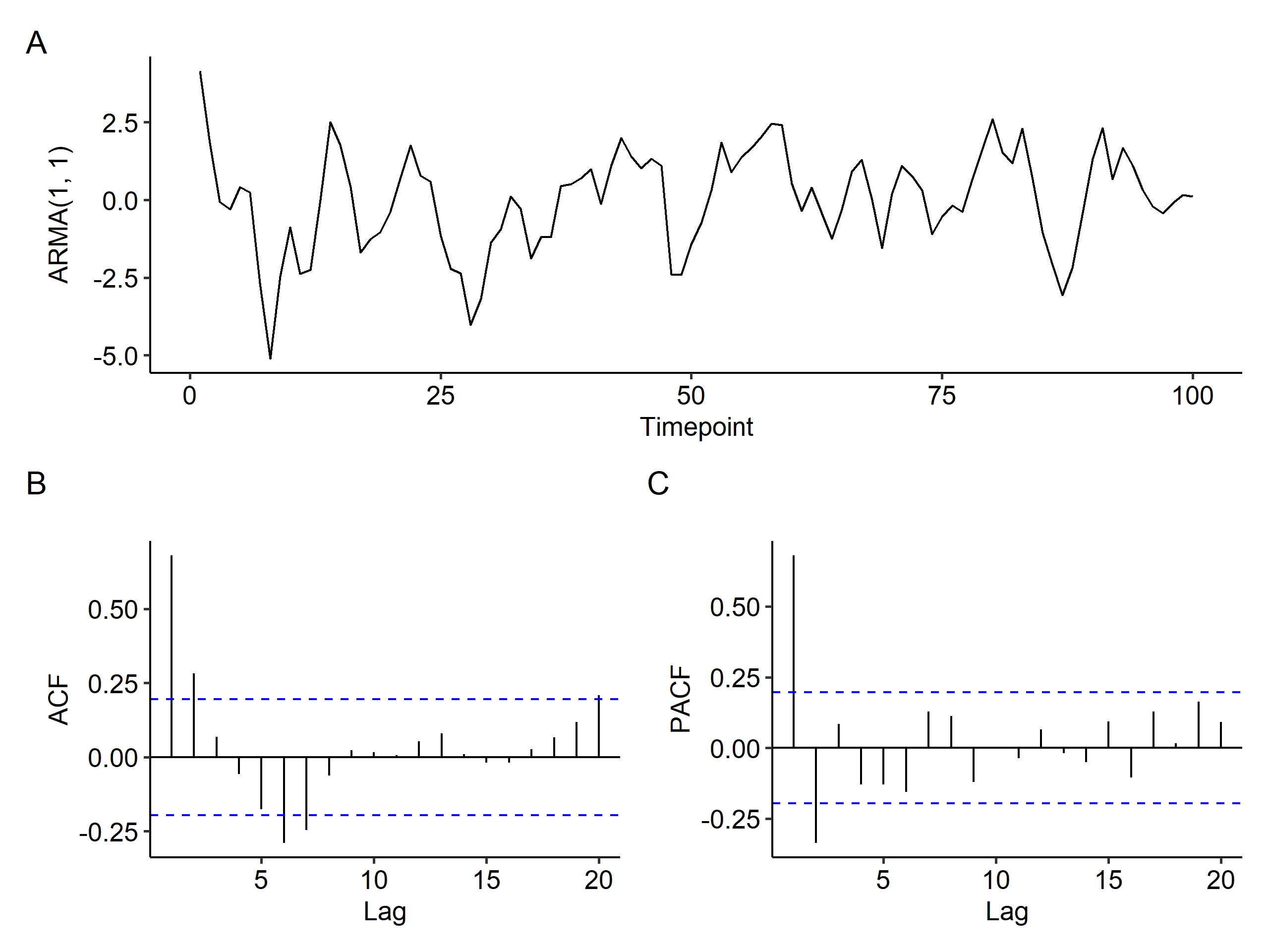
There’s no way to figure out the model from the time series plot. The ACF tails off (decays exponentially) as expected, but the PACF seems to have spikes at the first two lags and then cuts off - a feature of an AR(2) model. This tells us that it’s difficult to detect ARMA models.
ARMA(p, q)
The general expression for an ARMA(p, q) model is
$$ \begin{gathered} X_t = \underbrace{\phi_1 X_{t-1} + \phi_2 X_{t-2} + \cdots + \phi_p X_{t-p}}{AR(p)} + \underbrace{Z_t + \theta_1 Z{t-1} + \theta_2 Z_{t-2} + \cdots + \theta_q Z_{t-q}}{MA(q)} \\ X_t = \phi_1 X{t-1} - \phi_2 X_{t-2} = \cdots - \phi_p X_{t-p} = Z_t + \theta_1 Z_{t-1} + \theta_2 Z_{t-2} + \cdots + \theta_q Z_{t-q} \\ (1 - \phi_q B - \phi_2 B^2 - \cdots - \phi_p B^p)X_t = (1 + \theta_1 B + \theta_2 B^2 + \cdots + \theta_q B^q)Z_t \\ \Phi(B)X_t = \Theta(B)Z_t \end{gathered} $$
The ACF tails off to 0 after $q$ lags, and the PACF tails off to 0 after $p$ lags. We can think of this as overlaying the ACF and PACF plots from AR(p) and MA(q) models. Consider an ARMA(2, 1) process:
- AR(2): ACF tails off and PACF cuts off after lag 2.
- MA(1): ACF cuts off after lag 1 and PACF tails off.
- The ACF for the ARMA(2, 1) process will look like the ACF from an AR(2) model after lag 1, since the ACF for MA(1) cuts off to 0 after lag 1.
- The PACF for ARMA(2, 1) will look like the PACF from an MA(1) model after lag 2.
Stationarity and invertibility
For an AR(p) model
$$ X_t - \phi_1 X_{t-1} - \cdots - \phi_p X_{t-p} = Z_t, $$
if we express this using the AR polynomial, we get
$$ (1 - \phi_1 B - \cdots - \phi_p B^p)X_t = Z_t $$
The theory says if the solutions to the AR polynomial in $B$
$$ 1 - \phi_1 B - \cdots - \phi_p B^p = 0 $$
lies outside the unit circle, i.e. if all $|B| > 1$, we conclude AR(p) is stationary. 3 For example, the following model
$$ X_t = -1.2 X_{t-1} + Z_t $$
is not stationary because $|B| = \frac{1}{1.2} < 1$.
For the AR(2) model
$$ X_t = X_{t-1} - 0.24 X_{t-2} + Z_t, $$
we can express it as
$$ (1 - B + 0.24 B^2)X_t = Z_t $$
The solution for the AR polynomial is
$$ \begin{gathered} 1 - B + 0.24B^2 = 0 \\ B = \frac{1 \pm \sqrt{1 - 4 \times 0.24}}{2 \times 0.24} = \frac{1 \pm 0.2}{0.48} \end{gathered} $$
Since both solutions are greater than 1, the AR(2) process is stationary.
Similarly for an MA(q) model,
$$ \begin{aligned} X_t &= Z_t + \theta_1 Z_{t-1} + \cdots + \theta_q Z_{t-q} \\ &= (1 + \theta_1 B + \cdots + \theta_q B^q)Z_t \end{aligned} $$
If all solutions of $B$ for
$$ 1 + \theta_1 B + \cdots + \theta_q B^q = 0 $$
lies outside the unit circle, we conclude MA(q) is invertible (causal).
What about ARMA(p, q) models? For example,
$$ \begin{gathered} X_t = 0.8 X_{t-1} - 0.15 X_{t-2} + Z_t - 0.3 Z_{t-1} \\ (1 - 0.8B + 0.15 B^2)X_t = (1 - 0.3B)Z_t \end{gathered} $$
For stationarity of the above ARMA(2, 1) model, we only need to solve the AR polynomial:
$$ 1 - 0.8B + 0.15B^2 = 0 \Rightarrow |B| = \left|\frac{1}{0.3}\right|, \left|\frac{1}{0.5}\right| > 1, $$
so the model is stationary. For invertibility, we solve the MA polynomial:
$$ 1 - 0.3B = 0 \Rightarrow |B| = \left|\frac{1}{0.3} \right| > 1, $$
so the model is invertible.
Note that $B$ is an operator, so $X_t B$ is invalid. ↩︎
The model is $X_t - 0.5 X_{t-1} = Z_t + 0.5 Z_{t-1}$, or $(1 - 0.5B)(X_t - 0) = (1 + 0.5B)Z_t$.
↩︎1 2 3 4 5x <- arima.sim( list(order = c(1, 0, 1), ar = 0.5, ma = 0.5), n = 100 ) plot_time_series(x, x_type = "ARMA(1, 1)")If the solution for $B$ is complex, e.g. $a \pm b i$, then the condition for stationarity becomes $|B| = \sqrt{a^2 + b^2} > 1$. ↩︎
| Sep 04 | Moving Average Model | 6 min read |
| Aug 28 | Autoregressive Series | 9 min read |
| Nov 17 | Spectral Analysis | 9 min read |
| Nov 02 | Decomposition and Smoothing Methods | 14 min read |
| Sep 14 | Model Fitting and Forecasting | 15 min read |