Optimal Unbiased Estimator
The motivation here is to find the optimal estimator of $\theta$. Ideally, we want to find an estimator $\hat\theta_{opt}$ that minimizes the MSE: $$ \begin{equation} \label{eq:min-mse} MSE(\hat\theta_{opt}; \theta) \leq MSE(\hat\theta; \theta) \quad \forall \theta \in \Theta \end{equation} $$ for any estimator $\hat\theta$. Unfortunately, this is usually impossible. Recall when we had $Y_i \overset{i.i.d.}{\sim} Unif(0, \theta)$. For proposed estimators $\hat\theta_1 = 1$ and $\hat\theta_2 = \max(Y_1, \cdots, Y_n)$, if we plotted the two MSE curves:
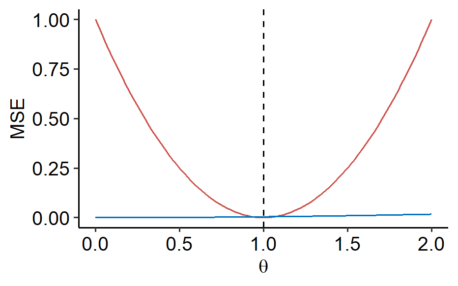
We can see that although $\hat\theta_1$ is a terrible estimator, it beats $\hat\theta_2$ at a narrow range around $1$.
To generalize the above, let $\theta_0$ be any fixed value of $\Theta$. Define estimator $\hat\theta = \theta_0$, then $MSE(\hat\theta; \theta_0) = 0$. For another estimator to beat this, it means $MSE(\hat\theta; \theta) = 0$ would have to be always true for $\theta \in \Theta$ in $\eqref{eq:min-mse}$.
Equation $\eqref{eq:min-mse}$ becomes solvable (and meaningful) when it is coupled with a constraint of unbiasedness.
Definition: An unbiased estimator $\hat\theta$ of $\theta$ is said to be Minimum Variance Unbiased Estimator (MVUE) if
$$
Var(\hat\theta; \theta) \leq (\hat\theta’; \theta) \quad \forall \theta \in \Theta
$$
for any unbiased estimator $\hat\theta$.
Review of conditional expectation and variance
For two random variables $X$ and $Y$, the expectation of $X$ given $Y$ is given as $$ E[X \mid Y] \rightarrow \begin{cases} \text{Compute } E[X \mid Y = y] = \sum_X xp(x \mid y) \text{ or } \int xf(x \mid y) \\ \text{Plug the random variable } Y \text{ into the function above} \end{cases} $$ In the end, this is random and the randomness comes from $Y$. Since $E[X \mid Y]$ is a random variable, we can take its expected value (which is known as the law of total expectation): $$ E\Big[E[X \mid Y] \Big] = E[X] $$ The conditional variance is defined similarly as above. The law of total variance states that $$ Var(X) = Var(E[X \mid Y]) + E[Var(X \mid Y)] $$
Rao-Blackwell theorem
Suppose $\hat\theta$ is unbiased for $\theta$, and its variance is finite: $Var(\hat\theta) < \infty$. Let $T$ be a sufficient statistic for $\theta$. Define a new estimator $\hat\theta^*$ where
$$ \hat\theta^* = E[\hat\theta \mid T] $$
The Rao-Blackwell theorem states that:
- $\hat\theta^*$ is still unbiased.
- $Var(\hat\theta^*; \theta) \leq Var(\hat\theta; \theta)$ for all $\theta \in \Theta$.
In practice, the variance is often much smaller than the original $\hat\theta$. The proof is given as follows.
By the law of total expectation, $$ E\left[E[\hat\theta \mid T]\right] = E[\hat\theta] = \theta $$
so $\hat\theta^*$ is unbiased. For the second statement,
$$ Var(\hat\theta) = Var\left(E[\hat\theta; T]\right) + E\left[Var(\hat\theta \mid T)\right] \geq Var\left(E[\hat\theta; T]\right) = Var(\hat\theta^*) $$
Note that even if $T$ is not sufficient, the arguments above still hold! So far we’re not using the second condition where $T$ ha to be sufficient. What’s missing here?
The key is that $\hat\theta^*$ has to be a statistic, which shouldn’t depend on the unknown $\theta$. By definition of sufficiency, the conditional distribution $\{(Y_1, \cdots, Y_n) \mid T\}$ doesn’t depend on $\theta$. Since $\hat\theta = f(Y_1, \cdots, Y_n)$, $\{\hat\theta \mid T\}$ doesn’t depend on $\theta$ as well. Therefore, $E[\hat\theta \mid T]$ doesn’t depend on $\theta$.
Remark: if what we’ve described above improves the estimator, why not do it again? $$ E[\hat\theta^* \mid T] = ? $$ Recall that if $X$ is a random variable and $f$ is a function, then $$ E[f(X) \mid X] = f(X) $$ Since $\hat\theta^$ is a function of $T$, $E[\hat\theta^ \mid T] = E[\hat\theta \mid T] = \hat\theta^$. In other words, we can’t further improve $\hat\theta^$.
Procedure to obtain good unbiased estimators
- Find a sufficient statistic $T$ for $\theta$, which can be done efficiently through the factorization theorem.
- Find a transform/function $f$ such that $\hat\theta = f(T)$ is unbiased for $\theta$, i.e.
$$ E[f(T)] = \theta \quad \forall \theta \in \Theta $$
Note that $\hat\theta$ is already a function of $T$, so $E[\hat\theta \mid T] = \hat\theta$. If an unbiased estimator of $\theta$ exists, then such a transform $f$ is step 2 always exists as well. The estimator $\hat\theta^*$ we introduced in the Rao-Blackwell theorem is a function of $T$ and satisfies the conditions above.
Bernoulli distribution example
Suppose $Y_i \overset{i.i.d.}{\sim} Bern(p)$. We know that $T = Y_1 + \cdots + Y_n$ is sufficient for $p$. We want to find $f$ such that $E[f(T)] = p$.
We know that $E[T] = np$, so it’s straightforward to make $f(T)$ unbiased: $f(t) = \frac{t}{n}$. $$ f(T) = \frac{Y_1 + \cdots + Y_n}{n} = \bar{Y}_n $$ and we may conclude that $\bar{Y}_n$ is the good unbiased estimator that we want to find through the procedure.
Exponential distribution example
Suppose $Y_i$ are an i.i.d. sample from PDF $$ f(y; \theta) = \begin{cases} \frac{1}{\theta}e^{-\frac{y}{\theta}}, & y \geq 0, \\ 0, & \text{otherwise} \end{cases} $$ where $\theta > 0$. $$ \begin{aligned} L(\theta) &= f(Y_1; \theta) \cdots f(Y_n; \theta) \\ &= \frac{1}{\theta^n} \exp \left( \frac{\sum_{i=1}^n Y_i}{\theta} \right) \\ &= g \times 1 \end{aligned} $$ By factorization, $T = \sum_{i=1}^n Y_i$ is a sufficient statistic. Next we want a transform $f$ such that $E[f(T)] = \theta$. $$ E[T] = E\left[ \sum_{i=1}^n Y_i \right] = nE[Y_1] = n\theta $$ This structure is exactly like what we saw in the previous example. We propose $f(t) = \frac{t}{n}$, so $f(T) = \bar{Y}_n$ is the good unbiased estimator.
“Good” is not good enough
Now we know how to find a “good” unbiased estimator. How can we go from here to the best unbiased estimator, namely MVUE?
Definition: A sufficient statistic $T$ for $\theta$ is said to be complete if the transform $f$ found in the procedure is unique.
Lehmann–Scheffé Theorem: If the sufficient statistic $T$ is complete, then $\hat\theta^* = f(T)$ in the procedure is the MVUE.
Proof: Suppose $\hat\theta$ is another unbiased estimator. Let $\tilde{f}(t) = E[\hat\theta \mid T]$. By the Rao-Blackwell theorem, $\tilde{f}(T)$ is unbiased. By the definition of completeness, $\tilde{f} = f$, so $$ \tilde{f}(T) = f(T) = \hat\theta^* $$ By the Rao-Blackwell theorem, $$ Var(\hat\theta^*) = Var(\tilde{f}(T)) \leq Var(\hat\theta) $$ In this course, we don’t check for completeness. When asked to find the MVUE, just apply the 2-step procedure.
Example
Suppose $Y_i \overset{i.i.d.}{\sim} Unif(0, \theta)$. We know $T = \max(Y_1, \cdots, Y_n)$ is sufficient for $\theta$, and that $$ E[T] = \frac{n}{n+1}\theta $$ We propose $f(t) = \frac{n+1}{n}t$, thus $$ f(T) = \frac{n+1}{n}\max(Y_1, \cdots, Y_n) $$ is the MVUE.
| Jan 30 | Sufficiency | 5 min read |
| Jan 29 | Maximum Likelihood Estimator | 7 min read |
| Jan 28 | The Method of Moments | 3 min read |
| Jan 27 | Consistency | 6 min read |
| Jan 25 | Bias and Variance | 11 min read |