Common Continuous Random Variables
The uniform distribution
In the discrete case, if the outcomes of a random experiment are equally likely, then calculating the probability of the events will be very easy. This “equally likely” idea may also be applied to continuous random variables.
Def: For a continuous random variable $X$, we say $X$ is uniformly distributed over the interval $(\alpha, \beta)$ if the density function of $X$ is
$$ f(X) = \begin{cases} \frac{1}{\beta - \alpha}, & \alpha \leq x \leq \beta \\ 0, & \text{otherwise} \end{cases} $$
In other words, the density function of $X$ is a constant over a given interval and zero otherwise. This holds because
$$ 1 = \int_{-\infty}^\infty f(x)dx = \int_\alpha^\beta Cdx = Cx \bigg|_\alpha^\beta = C(\beta - \alpha) $$ The plot for this function is a horizontal line at $\frac{1}{\beta - \alpha}$ between the interval $(\alpha, \beta)$, and $0$ otherwise. From $f(x)$, we can figure out the cumulative distribution function to be
$$ F(a) = \begin{cases} 0, & a < \alpha \\ \frac{a - \alpha}{\beta - \alpha}, & \alpha \leq a \leq \beta \\ 1, & a > \beta \end{cases} $$
Plotting $F(a)$ against $a$ would result in a line connecting $(\alpha, 0)$ and $(\beta, 1)$, and staying at $1$ onward.
Bus example
Buses arrive at a bus stop at a 15 minutes interval starting at 7:00 a.m. Suppose that a passenger arrives at this stop at a time that is uniformly distributed between 7 and 7:30. Find the probability that he needs to wait less than 5 minutes until the next bus arrives.
We know that buses are going to arrive at 7:00, 7:15 and 7:30 in this time interval. There are then two scenarios that the passenger waits less than 5 minutes: arriving between 7:10 and 7:15, or between 7:25 and 7:30. Define events $E_1 = {10 \leq X \leq 15}$ and $E_2 = {25 \leq X \leq 30}$.
$$ \begin{gather*} E = {\text{wait less than 5 minutes}} = E_1 \cup E_2 \\ P(E) = F(15) - F(10) + F(30) - F(25) \end{gather*} $$ Since $X \sim unif(0, 30)$, we have $$ F(a) = \begin{cases} 0, & a < 0 \\ \frac{a}{30}, & 0 \leq a \leq 30 \\ 1, & a > 30 \end{cases} $$ So $P(E) = \frac{1}{2} - \frac{1}{3} + 1 - \frac{5}{6} = \frac{1}{3}$.
Properties
We can get the expectation of $X \sim Unif(\alpha, \beta)$ directly from the definition. $$ \begin{aligned} E[X] &= \int_{-\infty}^\infty xf(x)dx \\ &= \int_\alpha^\beta x \frac{1}{\beta - \alpha}dx \\ &= \frac{1}{\beta - \alpha} \frac{x^2}{2} \bigg|\alpha^\beta \\ &= \frac{(\beta - \alpha)(\beta + \alpha)}{2(\beta - \alpha)} \\ &= \frac{\beta + \alpha}{2} \end{aligned} $$ Then we calculate $E[X^2]$ to find $Var(X)$. $$ \begin{aligned} E[X^2] &= \int\alpha^\beta \frac{x^2}{\beta - \alpha}dx \\ &= \frac{1}{\beta - \alpha} \frac{x^3}{3}\bigg|\alpha^\beta \\ &= \frac{\beta^3 - \alpha^3}{3(\beta - \alpha)} \\ &= \frac{(\beta - \alpha)(\beta^2 + \alpha\beta + \alpha^2)}{3(\beta - \alpha)} \\ &= \frac{\beta^2 + \alpha\beta + \alpha^2}{3} \\ Var(X) &= \frac{\beta^2 + \alpha\beta + \alpha^2}{3} - \left( \frac{\beta + \alpha}{2} \right)^2 \\ &= \frac{\beta^2 - 2\beta\alpha + \alpha^2}{12} \\ &= \frac{(\beta - \alpha)^2}{12} \end{aligned} $$ So we’ve found the expected value for the uniform distribution is $\frac{\beta + \alpha}{2}$, and the variance is $\frac{(\beta - \alpha)^2}{12}$. We also want to find the moment generating function for the uniform distribution. $$ \begin{aligned} M(t) &= E\left[e^{tX}\right] = \int{-\infty}^\infty e^{tx}f(x)dx \\ &= \int_\alpha^\beta \frac{1}{\beta - \alpha} e^{tx}dx \\ &= \frac{1}{\beta - \alpha} \frac{1}{t} \int_\alpha^\beta e^{tx}dtx \\ &= \frac{1}{t(\beta - \alpha)} e^{tx}\bigg|_\alpha^\beta \\ &= \frac{e^{t\beta} - e^{t\alpha}}{t(\beta - \alpha)} \end{aligned} $$
The normal distribution
Another very important type of continuous random variables is the normal random variable. The probability distribution of a normal random variable is called the normal distribution.
The normal distribution is the most important probability distribution in both theory and practice. In real world, many random phenomena obey, or at least approximate, a normal distribution. For example, the distribution of the velocity of the molecules in gas; the number of birds in flocks, etc.
Another reason for the popularity of the normal distribution is due to its nice mathematical properties. We first study the simplest case of the normal distribution, the standard normal distribution.
Standard normal distribution
Def: A continuous random variable $Z$ is said to follow a standard normal distribution if the density function of $Z$ is given by
$$ f(z) = \frac{1}{\sqrt{2\pi}} e^{-\frac{Z^2}{2}} \quad -\infty < z < \infty $$
Conventionally, we use $Z$ to denote a standard normal random variable, and $\Phi(z)$ to denote a standard normal distribution.
The density function of a normal random variable is a bell-shaped curve which is symmetric about its mean (in this case, $0$). The symmetry can be easily proven by $f(Z) = f(-Z)$. We can also find $f(0) = \frac{1}{\sqrt{2\pi}} \approx 0.4$. Next we prove this density function satisfies the properties of PDFs. The first property we want to prove is $$ \int_{-\infty}^\infty f(x)dx = \int_{-\infty}^\infty \frac{1}{\sqrt{2\pi}} e^{-\frac{z^2}{2}} dz = 1 $$ which is equivalent to proving $$ I = \int_{-\infty}^\infty e^{-\frac{x^2}{2}} dx = \sqrt{2\pi} $$ It’s easier to prove $I^2 = 2\pi$, as shown below: $$ \begin{equation} \label{eq:normal-i2} \begin{aligned} I^2 &= \int_{-\infty}^\infty e^{-\frac{x^2}{2}}dx \int_{-\infty}^\infty e^{-\frac{y^2}{2}}dy \\ &= \int_{-\infty}^\infty \int_{-\infty}^\infty e^{-\frac{x^2 + y^2}{2}}dxdy \end{aligned} \end{equation} $$ Intuitively, we can think of this as transforming a circle from Cartesian coordinates to polar coordinates, $dxdy = Jdrd\theta$.
In the Cartesian coordinate system the increase $dxdy$ can be thought as the area of a small rectangle. In the polar coordinate system, the increase in area can be approximated by a rectangle with one side being $dr$ and the other being the length of the arc when the angle increases by $d\theta$ and the radius is $r$. Thus, $dxdy = r drd\theta$. Now we have $$ \begin{cases} x^2 + y^2 = r^2 \\ \tan \theta = \frac{y}{x} \end{cases} \Rightarrow \begin{cases} x = r\cos \theta \\ y = r\sin \theta \end{cases} $$
So we can rewrite Equation $\eqref{eq:normal-i2}$ as
$$
\begin{aligned}
I^2 &= \int_0^\infty \int_0^{2\pi} e^{-\frac{r^2}{2}}rdrd\theta \\
&= -\int_0^\infty \int_0^{2\pi} e^{-\frac{r^2}{2}}d\left(-\frac{r^2}{2}\right) d\theta \\
&= -\int_0^{2\pi} d\theta \left( e^{-\frac{r^2}{2}} \right)\bigg|_0^\infty \\
&= -\int_0^{2\pi} d\theta (0 - 1) \\
&= \theta\bigg|_0^{2\pi} = 2\pi
\end{aligned}
$$
Formally speaking, the $J$ in $dxdy = Jdrd\theta$ is the Jacobian determinant, and can be found with
$$
J = \det \frac{\partial(x, y)}{\partial(r, \theta)} =
\begin{vmatrix}
\frac{\partial{x}}{\partial{r}} & \frac{\partial{x}}{\partial{\theta}} \\
\frac{\partial{y}}{\partial{r}} & \frac{\partial{y}}{\partial{\theta}}
\end{vmatrix}
$$
Knowing that $x = r \cos \theta$ and $y = r \sin\theta$, we can find the determinant of the Jacobian matrix
$$ \begin{aligned} J &= \begin{vmatrix} \cos\theta & r(-\sin\theta) \\ \sin\theta & r\cos\theta \end{vmatrix} \\ &= r\cos^2\theta + r\sin^2\theta = r \end{aligned} $$
Expectation and variance
We first find the expected value of a standard normal random variable. $$ \begin{aligned} E[X] &= \int_{-\infty}^\infty xf(x)dx = \int_{-\infty}^\infty x \cdot \frac{1}{\sqrt{2\pi}} e^{-\frac{x^2}{2}}dx \\ &= -\int_{-\infty}^\infty \frac{1}{\sqrt{2\pi}} e^{-\frac{x^2}{2}} d\left(-\frac{x^2}{2}\right) \\ &= -\frac{1}{\sqrt{2\pi}}\left( e^{-\frac{x^2}{2}} \right)\bigg|_{-\infty}^\infty = 0 \end{aligned} $$ and we can also get $E[X] = 0$ due to symmetry. To find the variance of $X$, we just need to find $E[X^2]$ since the expectation of $X$ is 0:
$$ \begin{aligned} E[X^2] &= \int_{-\infty}^\infty x^2f(x)dx = \int_{-\infty}^\infty x^2 \cdot \frac{1}{\sqrt{2\pi}} e^{-\frac{x^2}{2}}dx \\ &= -\int_{-\infty}^\infty \frac{1}{\sqrt{2\pi}} x e^{-\frac{x^2}{2}}d\left(-\frac{x^2}{2}\right) \\ &= -\frac{1}{\sqrt{2\pi}} \int_{-\infty}^\infty xd\left( e^{-\frac{x^2}{2}} \right) \end{aligned} $$ Recall integration by parts: $\int udv = \int duv - \int v du$. In our case $u = x$ and $v = e^{-\frac{x^2}{2}}$, so
$$ \begin{aligned} E[X^2] &= -\frac{1}{\sqrt{2\pi}} \left( \int_{-\infty}^\infty d\left( xe^{-\frac{x^2}{2}} \right) - \int_{-\infty}^\infty e^{-\frac{x^2}{2}}dx \right) \\ &= -\frac{1}{\sqrt{2\pi}} \left( xe^{-\frac{x^2}{2}}\bigg|_{-\infty}^\infty - \sqrt{2\pi} \right) \end{aligned} $$
When $x\rightarrow \infty$, $x$ goes to $\infty$ linearly, but $e^{-\frac{x^2}{2}}$ goes to $0$ exponentially, so the product goes to $0$. Similarly the term goes to $0$ when $x \rightarrow -\infty$. So we have
$$ E[X^2] = -\frac{1}{\sqrt{2\pi}} (-\sqrt{2\pi}) = 1 \Rightarrow Var(X) = 1- 0 = 1 $$
Cumulative probability function
The cumulative distribution function of a standard normal random variable is also very useful.
$$
\Phi(a) = F_Z(a) = \int_{-\infty}^a f(z)dz = \int_{-\infty}^a \frac{1}{\sqrt{2\pi}}e^{-\frac{z^2}{2}}dz
$$
Unfortunately, the integral has no analytical solution. People developed the standard normal table that can be used to find values for a given $a$. The table is referred as the $\Phi$ table or the $Z$ table. In R, we can use the pnorm() function.
For example, to find $F_Z(0.32)$ we first look for row $0.3$ and then find the column for $0.02$. Since the standard normal distribution is symmetric around $0$, $\Phi(-a)$ is equivalent to $1 - \Phi(a)$. There are also tables designed to describe $\Phi(a)$ through the right tail area.
In R, we can use the qnorm() function to find the corresponding quantiles.
| |

General normal distribution
So far we’ve been discussing the case $X \sim N(0, 1)$, the standard normal distribution. Now we extend our findings to a general case: $X \sim N(\mu, \sigma^2)$. The density function is given by $$ f(X) = \frac{1}{\sqrt{2\pi}\sigma}e^{-\frac{(x-\mu)^2}{2\sigma^2}} $$ The reason we focused on the standard normal distribution is because it’s easy to analyze. In addition, the properties of the general normal random variable can be derived from that of the standard normal random variable. If we consider a linear function of the standard normal random variable $Z$, $$ X = \mu + \sigma Z $$
we can easily find
$$ \begin{gather*} E[X] = E[\mu + \sigma Z] = \mu + \sigma E[Z] = \mu \\ Var(X) = Var(\mu + \sigma Z) + \sigma^2 Var(Z) = \sigma^2 \end{gather*} $$ In that sense, $$ X = \mu + \sigma Z \sim N(\mu, \sigma^2) $$ We can use this linear function to express $Z$ with $X$ and find the cumulative distribution function and probability density function of $X$:
$$ Z = \frac{X - \mu}{\sigma} \sim N(0, 1) $$
$$ \begin{gather*} F_X(a) = F_Z\left( \frac{a - \mu}{\sigma} \right) \\ f_X(X) = \frac{\partial F_X(a)}{\partial a} = \frac{\partial F_Z\left( \frac{a - \mu}{\sigma} \right)}{\partial a} \end{gather*} $$ Here we apply the chain rule to calculate the partial derivatives. Let $y = \frac{a - \mu}{\sigma}$,
$$ \begin{aligned} f_X(X) &= \frac{\partial F_Z(y)}{\partial y} \cdot \frac{\partial y}{\partial a} \\ &= \frac{1}{\sigma}f_Z \left( \frac{a - \mu}{\sigma} \right) \\ &= \frac{1}{\sigma} \cdot \frac{1}{\sqrt{2\pi}}e^{-\frac{\left( \frac{Z-\mu}{\sigma} \right)^2}{2}} \\ &= \frac{1}{\sqrt{2\pi}\sigma}e^{-\frac{(x-\mu)^2}{2\sigma^2}} \end{aligned} $$
and the cumulative distribution function
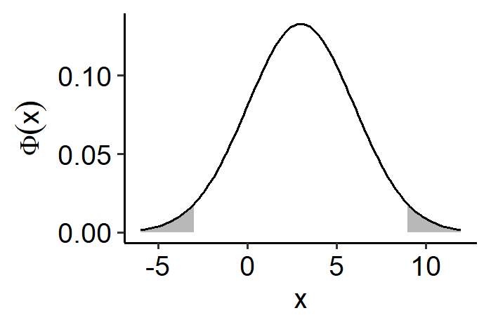
$$ F_X(a) = F_Z\left( \frac{a - \mu}{\sigma} \right) = \Phi\left( \frac{a - \mu}{\sigma} \right) $$ where the exact value can be found in the $\Phi$ table. For example, if $X \sim N(3, 9)$ and we want to find $P\{2 < X < 5\}$ and $P\{|X - 3| > 6\}$, we have $$ \frac{X - 3}{3} = Z \sim N(0, 1) $$
$$ \begin{aligned} P\{X \leq a\} &= F(a) = \Phi\left( \frac{a-3}{3} \right) \\ P\{2 < X < 5\} &= P\{X < 5\} - P\{X < 2\} \\ &= F_X(5) - F_X(2) \\ &= \Phi\left( \frac{2}{3} \right) - \Phi\left( -\frac{1}{3} \right) \\ &= \Phi\left( \frac{2}{3} \right) - 1 + \Phi\left( \frac{1}{3} \right) \approx 0.378 \\ P\{|X-3| >6\} &= P\{X-3 > 6\} + P\{ X - 3 < -6\} \\ &= P\{X > 9\} + P\{X < -3\} \\ &= 1 - F_X(9) + F_X(-3) \\ &= 1 - \Phi(2) + \Phi(-2) \\ &= 2(1 - \Phi(2)) \approx 0.046 \end{aligned} $$
Moment generating function
Again, we start with the simpler case of the standard normal distribution.
$$ \begin{equation}\label{eq:std-normal-mgf} \begin{aligned} M_Z(t) &= E[e^{tZ}] \\ &= \int_{-\infty}^\infty e^{tz}f(z)dz \\ &= \int_{-\infty}^\infty e^{tz} \frac{1}{\sqrt{2\pi}} e^{-\frac{z^2}{2}}dz \\ &= \frac{1}{\sqrt{2\pi}} \int_{-\infty}^\infty e^{tz - \frac{z^2}{2}} dz \\ &= \frac{1}{\sqrt{2\pi}} \int_{-\infty}^\infty e^{\frac{t^2 - (z-t)^2}{2}} dz \\ &= \frac{1}{\sqrt{2\pi}}e^{\frac{t^2}{2}} \int_{-\infty}^\infty e^{-\frac{(z-t)^2}{2}} dz \\ &= \frac{1}{\sqrt{2\pi}}e^{\frac{t^2}{2}} \int_{-\infty}^\infty e^{-\frac{(z-t)^2}{2}} d(z-t) \\ &= \frac{1}{\sqrt{2\pi}}e^{\frac{t^2}{2}} \sqrt{2\pi} \\ &= e^{\frac{t^2}{2}} \end{aligned} \end{equation} $$
We can validate this by calculating $E[Z]$ and $Var(Z)$ with the MGF. For the expectation,
$$ \begin{aligned} E[Z] &= M_Z^{(1)}(0) = \frac{de^{\frac{t^2}{2}}}{dt}\bigg|{t=0} \\ &= \frac{de^{\frac{t^2}{2}}}{d\frac{t^2}{2}} \cdot \frac{d\frac{t^2}{2}}{dt} \bigg|{t=0} \\ &= e^{\frac{t^2}{2}} t \bigg|_{t=0} = 0 \end{aligned} $$
And for the variance,
$$ \begin{aligned} Var(Z) &= E[Z^2] = M_t^{(2)}(0) \\ &= \frac{dM’(t)}{dt} \bigg|{t=0} \\ &= \frac{d\left[ e^{\frac{t^2}{2}} \right]}{dt} \\ &= e^{\frac{t^2}{2}} \frac{dt}{dt} + t \frac{de^{\frac{t^2}{2}}}{dt} \\ &= e^{\frac{t^2}{2}} + t \cdot te^{\frac{t^2}{2}} \\ &= (t^2 + 1)e^{\frac{t^2}{2}} \bigg|{t=0} = 1 \end{aligned} $$
Deriving the MGF of a general normal distribution requires a theorem: $X\ \sim N(\mu, \sigma^2)$, if $Y = a + bX$, we have
$$ M_Y(t) = e^{at}M_X(bt) $$ The proof is given as follows.
$$ \begin{aligned} M_Y(t) &= M_{a+bX}(t) \\ &= E\left[ e^{t(a+bX)} \right] \\ &= E\left[ e^{at} e^{tbX} \right] \\ &= e^{at}E\left[ e^{tbX} \right] \\ &= e^{at}M_X(bt) \end{aligned} $$
If we apply this to Equation $\eqref{eq:std-normal-mgf}$, we have $X \sim N(\mu, \sigma^2) = \mu + \sigma Z$, so
$$ M_X(t) = e^{\mu t}M_Z(\sigma t) = e^{\mu t} e^{\frac{\sigma^2t^2}{2}} = e^{\frac{\sigma^2t^2}{2} + \mu t} $$
Approximation to the binomial
Another very useful property of the normal distribution is that it can be used to approximate a binomial distribution when $n$ is very large.
Let $X$ be a binomial random variable with parameters $n$ and $p$. Denote $\mu$ and $\sigma$ the mean and standard deviation of $X$. Then we have the normal approximation to the binomial
$$ P\left\{\frac{X - \mu}{\sigma} \leq a\right\} \rightarrow \Phi(a) \quad \text{as } n \rightarrow \infty $$ where $\Phi(\cdot)$ is the distribution function of $Z \sim N(0, 1)$, i.e. $\Phi(a) = P{Z \leq a}$. In other words, when $n \rightarrow \infty$, $\frac{X - \mu}{\sigma} \rightarrow Z$. We also know that
$$ \begin{gather*} E[X] = np = \mu \\ Var(X) = np(1-p) = \sigma^2 \end{gather*} $$
so we can rewrite the equation as
$$ P\left\{ \frac{X - np}{\sqrt{np(1-p)}} \leq a \right\} \rightarrow \Phi(a) \quad \text{as } n \rightarrow \infty $$ The proof of this theorem is a special case of the central limit theorem, and we’ll discuss it in a later chapter.
There’s another approximation to the binomial distribution: the Poisson approximation, and its conditions are complementary to the conditions of the normal approximation. The Poisson approximation requires $n$ to be large ($ n \geq 20$) and $p$ to be small ($p \leq 0.05$) such that $np = \lambda$ is a fixed number.
The normal approximation is reasonable when $n$ is very large and $p$ and $1-p$ are not too small, i.e. $p \neq 0$ and $p \neq 1$.
We’ll demonstrate the approximation with an example. Suppose that we flip a fair coin 40 times, and let $X$ denote the number of heads observed. We want to calculate $P\{X = 20\}$.
We have $X \sim Bin(40, 0.5)$. We can calculate the probability directly:
$$ P\{X = 20\} = \binom{40}{20} 0.5^{20}(1 - 0.5)^{20} \approx 0.1254 $$ We can also apply the normal approximation. we can
$$ \begin{gather*} \mu = np = 20 \\ \sigma = \sqrt{Var(X)} = \sqrt{np(1-p)} = \sqrt{10} \end{gather*} $$ Since we’re approximating a discrete distribution with a continuous one, we need a range instead of an exact value:
$$ \begin{aligned} P\{X = 20\} &= P\{19.5 \leq X \leq 20.5\} \quad \text{because X is discrete} \\ &= P\left\{ \frac{19.5 - 20}{\sqrt{10}} \leq \frac{X - 20}{\sqrt{10}} \leq \frac{20.5 - 20}{\sqrt{10}} \right\} \\ &\approx P\left\{ -0.16 \leq \frac{X - 20}{\sqrt{10}} \leq 0.16 \right\} \\ &= \Phi(0.16) - \Phi(-0.16) \\ &= 2\Phi(0.16) - 1 \approx 0.1272 \end{aligned} $$
The numbers turn out to be fairly close. The normal approximation becomes much more useful when the probability of the binomial can’t be easily directly calculated. Suppose the ideal class size of a college is 150 students. The college knows from past experience that, on average, only 30 of students will accept their offers. If the college gives out 450 offers, what is the probability that more than 150 students will actually attend?
For simplicity, we assume the decision of the students is independent from each other. Let $X$ be the number of students who accept the offer. $X \sim Bin(450, 0.3)$. $$ P\{X > 150\} = 1 - P\{X \leq 150\} = 1 - \sum_{i=0}^{150}P_X(i) $$ We can see that it’s hard to calculate this probability by hand. Again, we can apply the normal approximation. We have $\mu = np = 450 \times 0.3 = 135$ and $\sigma = \sqrt{np(1-p)} = \sqrt{94.5}$.
$$ \begin{aligned} P\{X > 150\} &= P\{ X \geq 150.5 \} \\ &= \left\{ \frac{X - \mu}{\sigma} \geq \frac{150.5 - \mu}{\sigma} \right\} \\ &= 1 - \Phi\left( \frac{150.5 - \mu}{\sigma} \right) \approx 0.0559 \end{aligned} $$
The exponential distribution
Def: A continuous random variable $X$ is an exponential random variable with parameter $\lambda$ if the density function is given by
$$ f(X) = \begin{cases} \lambda e^{-\lambda X}, & X \geq 0 \\ 0, & X < 0 \end{cases} $$ where $\lambda > 0$. In practice, the exponential distribution often arises as the distribution of the amount of time until some specific event occurs. For example, the lifetime of a new mobile phone; the amount of time from now until an earthquake occurs; the survival time of a patient.
Properties
If $X \sim Exp(\lambda)$,
$$ \begin{aligned} F_X(a) &= P{X \leq a} \\ &= \int_{-\infty}^a f(x)dx \\ &= \int_0^a f(x)dx \quad \text{if } a > 0 \\ &= \int_0^a \lambda e^{-\lambda x}dx \\ &= -\int_0^a e^{-\lambda x} d(-\lambda x) \\ &= -e^{-\lambda x} \bigg|_0^a \\ &= 1 - e^{-\lambda a} \end{aligned} $$
Cleaning this up a bit, we have the PDF of $X$ as
$$ F_X(a) = \begin{cases} 1 - e^{-\lambda a}, & a \geq 0 \\ 0, & a < 0 \end{cases} $$
To find the expectation of $X$, we first prove that
$$ E[X^n] = \frac{n}{\lambda} E[x^{n-1}] $$
$$ \begin{aligned} E[X^n] &= \int_0^\infty x^n\lambda e^{-\lambda x} dx \\ &= -\int_0^\infty x^n d(e^{-\lambda x}) \\ &= -\left( x^n e^{-\lambda x} \bigg|0^\infty - \int_0^\infty e^{-\lambda x}d(x^n) \right) \\ &= -\left(\lim{x \rightarrow \infty} \frac{x^n}{e^{\lambda x}} - 0 - \int_0^\infty nx^{n-1}e^{-\lambda x}dx \right) \\ &= \frac{n}{\lambda} \int_0^\infty x^{n-1}\lambda e^{-\lambda x} dx \\ &= \frac{n}{\lambda} E[X^{n-1}] \end{aligned} $$ Now we can easily find $E[X]$ by setting $n=1$:
$$ E[X] = \frac{1}{\lambda} E[X^{1-1}] = \frac{1}{\lambda} $$ We also have
$$ E[X^2] = \frac{2}{\lambda}E[X] = \frac{2}{\lambda^2} $$
so the variance of $X$ is
$$ Var(X) = \frac{2}{\lambda^2} - \frac{1}{\lambda^2} = \frac{1}{\lambda^2} $$ Finally, the moment generating function of $X$ is
$$ \begin{aligned} M_X(t) &= E\left[ e^{tx} \right] \\ &= \int_{-\infty}^\infty e^{tx}f(x)dx \\ &= \int_0^\infty e^{tx} \lambda e^{-\lambda x}dx \\ &= \lambda \int_0^\infty e^{(t-\lambda)x}dx \\ &= \frac{\lambda}{t - \lambda} \int_0^\infty e^{(t-\lambda)x}d(t - \lambda)x \\ &= \frac{\lambda}{t - \lambda} e^{(t - \lambda)x} \bigg|_0^\infty \quad \text{, let } t < \lambda \\ &= \frac{\lambda}{\lambda - t} \end{aligned} $$ The MGF is given by
$$ M_X(t) = \begin{cases} \frac{\lambda}{\lambda - t}, & t < \lambda \\ \text{not defined}, & t \geq \lambda \end{cases} $$
Memoryless
The exponential probability is usually defined as a probability associated with the time counted from now and onward. So why don’t we care about what happened in the past?
For example, when we consider the time from now to the next earthquake, why don’t we care about how long has it been since the last earthquake? This leads to a nice property the exponential distribution has.
Def: We say a non-negative random variable $X$ is memoryless if
$$ P\{X > s + t \mid X > t\} = P\{X > s\} \quad \forall s, t \geq 0 $$
Going back to the earthquake example, the memoryless property means that the probability we will not observe an earthquake for $t+s$ days given that it has already been $t$ days without an earthquake is the same as the probability of not observing an earthquake in the first $s$ days.
$$ \begin{aligned} P\{X > s + t \mid X > t\} &= \frac{P\{ X > s + t, x > t \}}{P\{ x > t \}} \\ &= \frac{P\{X > s + t\}}{P\{ x > t \}} \\ P\{X > s + t\} &= P\{X > t\}P\{X > s\} \end{aligned} $$ if X is memoryless. For the exponential distribution,
$$ \begin{aligned} P\{X > s + t\} &= 1 - F(s + t) \\ &= 1 - \left[ 1 - e^{-\lambda(s + t)} \right] \\ &= e^{-\lambda(s + t)} \\ &= e^{-\lambda t} e^{-\lambda s} \\ &= \left[ 1 - e^{-\lambda t} \right]\left[ 1 - e^{-\lambda s} \right] \\ &= (1 - F(t))(1 - F(s)) \\ &= P(X > t)P(X > s) \end{aligned} $$
There’s various continuous distributions that are very important but not included here, such as the beta distribution and the gamma distribution. In fact, the exponential distribution and the chi-square distribution are both special cases of the gamma distribution. Proofs and properties of these distributions might be included in a later chapter.
| Dec 28 | Sampling Distribution and Limit Theorems | 6 min read |
| Dec 08 | Functions of Random Variables | 14 min read |
| Nov 06 | Multivariate Probability Distributions | 23 min read |
| Oct 06 | Definitions for Discrete Random Variables | 7 min read |
| Oct 06 | Common Discrete Random Variables | 14 min read |