Linear Space of Matrices

In the previous two sections (vector space and geometrical considerations) we’ve been focusing on vector operations and properties. Now we’re ready to come back to matrices. Associated with any matrix is a very important characteristic called the rank. There are several (consistent) ways of defining the rank. The most fundamental of these is in terms of the dimension of a linear space.
Definitions
Recall a matrix $\boldsymbol{A}: m \times n$ has $\boldsymbol{a}_1, \cdots, \boldsymbol{a}_n \in \mathbb{R}^m$ columns and $\boldsymbol{\alpha}_1^\prime, \cdots, \boldsymbol{\alpha}_m^\prime \in \left( \mathbb{R}^n \right)^\prime$ rows. The column space of $\boldsymbol{A}$ contains all linear combinations of the columns:
$$ \begin{aligned} \mathcal{C}(\boldsymbol{A}) &= \mathcal{L}(\boldsymbol{a}_1, \cdots, \boldsymbol{a}_n) \\ &= \left\{ \sum_{j=1}^n c_j \boldsymbol{a}_j, \quad c_j \in \mathbb{R} \right\} \\ &= \{ \boldsymbol{Ac}, \quad \boldsymbol{c} \in \mathbb{R}^n \}, \quad \boldsymbol{c} = (c_1, \cdots, c_n)^\prime \end{aligned} $$
This means for any $\boldsymbol{y} \in \mathcal{C}(\boldsymbol{A})$, there exists $\boldsymbol{x} \in \mathbb{R}^n$ such that $\boldsymbol{y} = \boldsymbol{Ax}$.
Similarly, the row space of $\boldsymbol{A}$ is
$$ \begin{aligned} \mathcal{R}(\boldsymbol{A}) &= \mathcal{L}(\boldsymbol{\alpha}_1^\prime, \cdots, \boldsymbol{\alpha}_m^\prime) \\ &= \left\{ \sum_{i=1}^m c_i \boldsymbol{\alpha}_j^\prime, \quad c_i \in \mathbb{R} \right\} \\ &= \{ \boldsymbol{c}^\prime \boldsymbol{A}, \quad \boldsymbol{c} \in \mathbb{R}^m \} \end{aligned} $$
Note that
$$ \begin{gathered} \boldsymbol{y} \in \mathcal{C}(\boldsymbol{A}) \Longleftrightarrow \boldsymbol{y}^\prime \in \mathcal{R}(\boldsymbol{A}^\prime) \\ \boldsymbol{x}^\prime \in \mathcal{R}(\boldsymbol{A}) \Longleftrightarrow \boldsymbol{x} \in \mathcal{C}(\boldsymbol{A}^\prime) \end{gathered} $$
Properties
$dim(\mathcal{C}(\boldsymbol{A})) \leq \min(n, m)$. The dimension of the column space of $\boldsymbol{A}$ is called the
rankof $\boldsymbol{A}$, which is written as $rank(\boldsymbol{A}) \triangleq r(\boldsymbol{A})$.$dim(\mathcal{R}(\boldsymbol{A})) = dim(\mathcal{C}(\boldsymbol{A})) = r(\boldsymbol{A})$, which implies the number of LIN columns is equal to the number of LIN rows.
Proof: Show that the row rank is equal to the column rank. Let $r$ denote the row rank, that is we have $r$ linearly independent rows. This means $\mathcal{R}(\boldsymbol{A})$ has a basis $\{\boldsymbol{x}_1^\prime, \cdots, \boldsymbol{x}_r^\prime\}$. We will show that $\{\boldsymbol{Ax}_1, \cdots, \boldsymbol{Ax}_r\}$ is linearly independent.
We show this because each vector $\boldsymbol{Ax}_i \in \mathcal{C}(\boldsymbol{A})$. If we can show the set is linearly independent, then the dimension of the column space has to be at least $r$. To show this, we set
$$ \sum_{i=1}^r c_i \boldsymbol{Ax}_i = \boldsymbol{0} $$
where the $c_i$’s are scalars. If we take $\boldsymbol{A}$ outside,
$$ \boldsymbol{A} \left( \sum_{i=1}^r c_i \boldsymbol{x}_i \right) = \boldsymbol{0} $$
Let $\boldsymbol{v} = \sum_{i=1}^r c_i \boldsymbol{x}_i$. If $\boldsymbol{Av} = \boldsymbol{0}$, then $\boldsymbol{v}^\prime$ has to be orthogonal to each row of $\boldsymbol{A}$, which means $\boldsymbol{v}^\prime \perp \mathcal{R}(\boldsymbol{A})$. Note that $\boldsymbol{v}^\prime$ is a linear combination of the rows of $\boldsymbol{A}$, so $\boldsymbol{v}^\prime \in \mathcal{R}(\boldsymbol{A})$. The only vector that belongs to a subspace and is orthogonal to that subspace is the zero vector.
If $\boldsymbol{v} = \boldsymbol{0}$, then $c_i = 0$ for all $i$ because the $\boldsymbol{x}_i$’s are linearly independent. Thus, the $\boldsymbol{Ax}_i$’s are linearly independent. The column space of $\boldsymbol{A}$ has a set of $r$ linearly independent vectors, so $dim(\mathcal{C}(\boldsymbol{A})) \geq r$.
We can repeat the above argument with $c \triangleq dim(\mathcal{C}(\boldsymbol{A}))$, and show that $dim(\mathcal{R}(\boldsymbol{A})) \geq c$. By showing both sides of the inequality, we arrive at the conclusion that $r=c$, i.e. the dimension of the column space is the same as the dimension of the row space, and that’s what we call the rank of $\boldsymbol{A}$.
If $r(\boldsymbol{A}) = m$, then we say $\boldsymbol{A}$ has full row rank1. If $r(\boldsymbol{A}) = n$, then we say $\boldsymbol{A}$ has full column rank. Either case, we say $\boldsymbol{A}$ has
full rank. If a matrix is not of full rank, it isrank-deficient.If $r(\boldsymbol{A}) = r$, then there exists matrix $\boldsymbol{B}: m \times r$, $r(\boldsymbol{B}) = r$ (full column rank) and matrix $\boldsymbol{T}: r \times n$, $r(\boldsymbol{T}) = r$ (full row rank), such that $\boldsymbol{A} = \boldsymbol{BT}$.
Any matrix can be written as a product of two full rank matrices. $\mathcal{C}(\boldsymbol{A})$ has $r$ basis vectors, and we can put them into an $m \times r$ matrix $\boldsymbol{B}$. Each column of $\boldsymbol{A}$, $\boldsymbol{a}_i$, is in $\mathcal{C}(\boldsymbol{A})$, so $\boldsymbol{a}_i$ can be expressed as $\boldsymbol{a}_i = \boldsymbol{By}_i$ where the $\boldsymbol{y}_i$’s are $r \times 1$ vectors, and we can put them together into an $r \times n$ matrix $\boldsymbol{T}$.
$r(\boldsymbol{AB}) \leq \min(r(\boldsymbol{A}), r(\boldsymbol{B}))$ for any $\boldsymbol{A}$, $\boldsymbol{B}$ matrices.
Proof: We first show that $r(\boldsymbol{AB}) \leq r(\boldsymbol{A})$ from the fact that $\mathcal{C}(\boldsymbol{AB}) \subset \mathcal{C}(\boldsymbol{A})$. Note that
$$ \boldsymbol{AB} = [\boldsymbol{Ab}_1, \cdots, \boldsymbol{Ab}_q] $$
where $\boldsymbol{B}$ has $q$ columns. Each column of $\boldsymbol{AB}$ has a form of $\boldsymbol{Ab}_i$, which is in $\mathcal{C}(\boldsymbol{A})$. In other words, any vector that lives in the column space of $\boldsymbol{AB}$ is in the column space of $\boldsymbol{A}$.
Similarly, we can show $r(\boldsymbol{AB}) \leq r(\boldsymbol{B})$ from the fact that $\mathcal{R}(\boldsymbol{AB}) \subset \mathcal{R}(\boldsymbol{B})$2.
If an $m \times n$ matrix $\boldsymbol{A}$ with rank $r$ is written as $\boldsymbol{A} = \boldsymbol{BT}$ with $\boldsymbol{B}: m \times r$ and $\boldsymbol{T}: r \times n$, then $r(\boldsymbol{B}) = r(\boldsymbol{T}) = r$.
This means both $\boldsymbol{B}$ and $\boldsymbol{T}$ have full rank, specifically $\boldsymbol{B}$ has full column rank and $\boldsymbol{T}$ has full row rank. This is true because
$$ r = r(\boldsymbol{A}) = r(\boldsymbol{BT}) \leq r(\boldsymbol{B}) \leq r \Rightarrow r(\boldsymbol{B}) = r $$
The
null spaceof $\boldsymbol{A}: m \times n$ is the collection of $n \times 1$ vectors that such that$$ N(\boldsymbol{A}) = \{\boldsymbol{x} \mid \boldsymbol{Ax} = \boldsymbol{0}\} $$
The null space is a subspace in $\mathbb{R}^n$. If $\boldsymbol{x} \in N(\boldsymbol{A})$, $\boldsymbol{x}$ is orthogonal to each row of $\boldsymbol{A}$, thus
$$ N(A) = \mathcal{R}(A)^\perp $$
A square matrix $\boldsymbol{A}: n \times n$ with rank $n$ is called
non-singular. If $r(\boldsymbol{A}) < n$, it issingular.For matrices $\boldsymbol{A}: m \times n$ and $\boldsymbol{B}: m \times q$, the
horizontal concatenationof $\boldsymbol{A}$ and $\boldsymbol{B}$ is an $m \times (n+q)$ matrix denoted $[\boldsymbol{A}, \boldsymbol{B}]$. Since $\mathcal{C}(\boldsymbol{A}) \subset \mathcal{C}([\boldsymbol{A}, \boldsymbol{B}])$, we have $r(\boldsymbol{A}) \leq r([\boldsymbol{A}, \boldsymbol{B}])$.$r([\boldsymbol{A}, \boldsymbol{B}]) \leq r(\boldsymbol{A}) + r(\boldsymbol{B})$. Think in terms of linearly independent columns.
$\mathcal{C}(\boldsymbol{A} + \boldsymbol{B}) \subset \mathcal{C}([\boldsymbol{A}, \boldsymbol{B}])$. The reason is
$$ \begin{gathered} \mathcal{C}(\boldsymbol{A} + \boldsymbol{B}) = \{ (\boldsymbol{A} + \boldsymbol{B})\boldsymbol{x} = \boldsymbol{Ax} + \boldsymbol{Bx} \} \\ \mathcal{C}([\boldsymbol{A}, \boldsymbol{B}]) = \left\{ [\boldsymbol{A}, \boldsymbol{B}]\begin{pmatrix} \boldsymbol{y}_1 \\ \boldsymbol{y}_2 \end{pmatrix} = \boldsymbol{Ay}_1 + \boldsymbol{By}_2 \right\} \end{gathered} $$
From this we can see that
$$ r(\boldsymbol{A} + \boldsymbol{B}) \leq r([\boldsymbol{A}, \boldsymbol{B}]) \leq r(\boldsymbol{A}) + r(\boldsymbol{B}) $$
$\mathcal{C}(\boldsymbol{A}^\prime \boldsymbol{A}) = \mathcal{C}(\boldsymbol{A}^\prime)$, and $\mathcal{C}(\boldsymbol{AA}^\prime) = \mathcal{C}(\boldsymbol{A})$. Similarly for the row spaces,
$$ \mathcal{R}(\boldsymbol{A}^\prime \boldsymbol{A}) = \mathcal{R}(\boldsymbol{A}), \quad \mathcal{R}(\boldsymbol{AA}^\prime) = \mathcal{R}(\boldsymbol{A}^\prime) $$
and the ranks:
$$ r(\boldsymbol{A}^\prime \boldsymbol{A}) = r(\boldsymbol{A}) = r(\boldsymbol{AA}^\prime) = r(\boldsymbol{A}^\prime) $$
Projection
Recall that in Projection to a subspace we showed that $P(\boldsymbol{x} \mid \mathcal{V})$ has the shortest distance to $\boldsymbol{x}$ among all $\boldsymbol{y} \in \mathcal{V}$, i.e. for any $\boldsymbol{y} \in \mathcal{V}$,
$$ \|\boldsymbol{y} - \boldsymbol{x}\|^2 \geq \| P(\boldsymbol{x} \mid \mathcal{V}) - \boldsymbol{x} \|^2 $$
The statistical application for this is that suppose we have data $\boldsymbol{y} = (y_1, \cdots, y_n)^\prime$, and our goal is to explain or predict $\boldsymbol{y}$ using another variable $\boldsymbol{x} = (x_1, \cdots, x_n)^\prime$.
In simple linear regression (SLR), we find $\beta_0$ and $\beta_1$ such that $\beta_0 + \beta_1 \boldsymbol{x}$ best explains $\boldsymbol{y}$. In other words, we find the vector in the subspace
$$ \mathcal{V} = \{ \beta_0 \boldsymbol{1}_n + \beta_1 \boldsymbol{x} \mid \beta_0, \beta_1 \in \mathbb{R} \} $$
that is closest to $\boldsymbol{y}$.
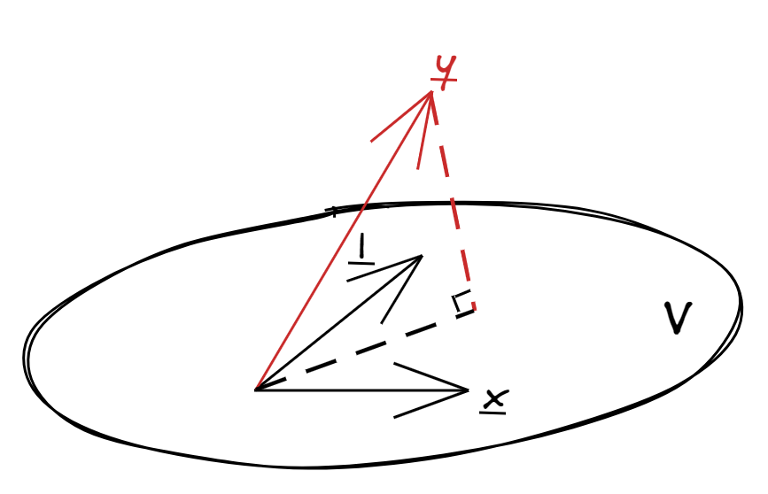
So how do we find the projection $P(\boldsymbol{y} \mid \mathcal{V})$? $\{ \boldsymbol{1}_n, \boldsymbol{x} \}$ is a basis.
By definition, we have
$$ \begin{gathered} P(\boldsymbol{y} \mid \mathcal{V}) = \beta_0 \boldsymbol{1}_n + \beta_1 \boldsymbol{x} \\ \begin{cases} \boldsymbol{y} - (\beta_0 \boldsymbol{1}_n + \beta_1 \boldsymbol{x}) \cdot \boldsymbol{1}_n = 0 \\ \boldsymbol{y} - (\beta_0 \boldsymbol{1}_n + \beta_1 \boldsymbol{x}) \cdot \boldsymbol{x} = 0 \end{cases} \Rightarrow \begin{cases} \boldsymbol{y}^\prime \boldsymbol{1}_n - \beta_0 n - \beta_1 \boldsymbol{x}^\prime \boldsymbol{1}_n = 0 \\ \boldsymbol{y}^\prime \boldsymbol{x} - \beta_0 \boldsymbol{x}^\prime \boldsymbol{1}_n - \beta_1 \boldsymbol{x}^\prime \boldsymbol{x} = 0 \end{cases} \\ \hat\beta_0 = \bar{y} - \beta_1 \bar{x} \\ \hat\beta_1 = \frac{\sum (x_i - \bar{x})(y_i - \bar{y})}{\sum(x_i - \bar{x})^2} = \frac{S_{xy}}{S_{xx}} \end{gathered} $$
What we have here is
$$ \hat{y} = \hat\beta_0 + \hat\beta_1 \boldsymbol{x} $$
which is the projection of $\boldsymbol{y}$ onto $\mathcal{V}$. To ensure that $\boldsymbol{1}_n$ and $\boldsymbol{x}$ are orthogonal, we can use Gram-Schmidt orthogonalization:
$$ \boldsymbol{1}_n, \boldsymbol{x} \xrightarrow{G-S} \boldsymbol{1}_n, \boldsymbol{x} - \bar{x}\boldsymbol{1}_n = \begin{pmatrix} x_1 - \bar{x} \\ \vdots \\ x_n - \bar{x} \end{pmatrix} $$
| Oct 12 | Matrix Inverse | 6 min read |
| Sep 21 | Projection | 7 min read |
| Sep 14 | Definitions in Arbitrary Linear Space | 6 min read |
| Aug 31 | Vector Space | 8 min read |
| Nov 18 | Eigenvalues and Eigenvectors | 20 min read |