Bayesian Inference for the Normal Model

This lecture discusses Bayesian inference of the normal model, most commonly used for continuous data. The normal distribution has two parameters (corresponding to mean and variance), and so while we will ultimately discuss posterior inference for multiple parameters, we focus on posterior estimation of a single parameter in this lecture – in particular, estimating the mean given a fixed variance.
The example we’re going to study is about crab shells. Two scientists1 were interesting in studying mophological variation of Leptograpsus variegatus, also known as the purple rock crab. They collected $n=200$ crabs and measured their shape through 5 variables. Our focus will be on carapace length (in mm), the length of the crab’s protective upper shell. The goal is to estimate the typocal carapace length, as well as the variability in lengths.
Exploratory data analysis
The dataset can be obtained from the MASS R package. The crabs data frame has 200 rows and 8 columns, describing 5 morphological measurements on 50 crabs each of two color forms and both sexes.
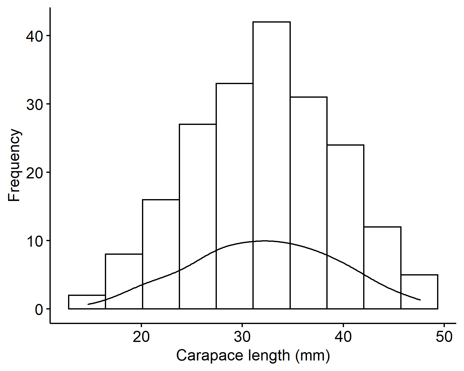
From the histogram of the carapace lengths2, we can see the values range from 10 to 50 millimeters and is centered around 30mm. The mean is 32.11mm and the variance is 50.68mm$^2$. The distribution looks overall symmetric with no outliers.
Sampling model
Let $Y$ be a random variable representing the carapace length (for one of the crabs). The normal model is often used for continuous quantities which are distributed symmetrically with few outliers:
The parameters of interest are $\theta$, the true average carapace length (in mm); and $\sigma^2$, the true variance in carapace length (in mm$^2$). The probability density function is:
Like the Poisson model, our data actually consists of $n=200$ observations, each representing the carapace length of a different crab. We will assume that each observation is conditionally independent:
This means if $\boldsymbol{Y} = (Y_1, \cdots, Y_n)$, then
Estimation of multiple parameters
This is the first model where we want to estimate multiple parameters. There are two ways to approach inference:
Assume one parameter is known, and compute the posterior for the other parameter. This is an overly simplistic view, but this is our focus in this lecture.
When $\theta$ is unknown and $\sigma^2$ is known, we fix $\sigma^2$:
$$ p(\theta \mid y, \sigma^2) \propto p(y \mid \theta, \sigma^2) p(\theta) $$When $\theta$ is known and $\sigma^2$ is unknown:
$$ p(\sigma^2 \mid y, \theta) \propto p(y \mid \theta, \sigma^2) p(\sigma^2) $$Assume both parameters are unknown, and compute a joint posterior for $(\theta, \sigma^2)$:
$$ p(\theta, \sigma^2 \mid y) \propto p(y \mid \theta, \sigma^2) p(\theta, \sigma^2) $$We will discuss this two-dimensional prior case in later lectures.
Prior model for $\theta$
For the rest of this lecture, we assume that the scientist is extremely confident that the true variance $\sigma^2 = 45 mm^2$, i.e. we will treat this value as fixed and known. In this case, we only need to specify a prior model for $\theta$, the average carapace length. One suitable choice is:
where $\mu_0$ is chosen as the “center” of the prior beliefs, and $\tau_0^2$ reflects uncertainty in prior beliefs. As we increase $\tau_0^2$, the distribution becomes more spread out. The probability density function for the prior distribution is:
By Bayes’ Theorem, the posterior can be computed:
To make this into a kernel of a normal distribution, we want it to be in the form:
We can find that the posterior follows $N(\mu_n, \tau_n^2)$, where
and $\mu_n$ is found from its ratio with $\tau_n^2$ in the second term.
Prior hyperparameter selection for $\theta$
Suppose we are very confident based on previous studies that the average carapace length is somewhere between 12 and 44 mm. How can we select the prior hyperparameters $\mu_0$ and $\tau_0^2$?
With this prior belief, it makes sense to set the center at the middle of 12 and 44 mm, and that midpoint is 28mm. Now the question is how much uncertainty should be associated with the prior here. If we are 95% confident, then going at 2 standard deviations from $\mu_0$ gives us 95% of the probability:
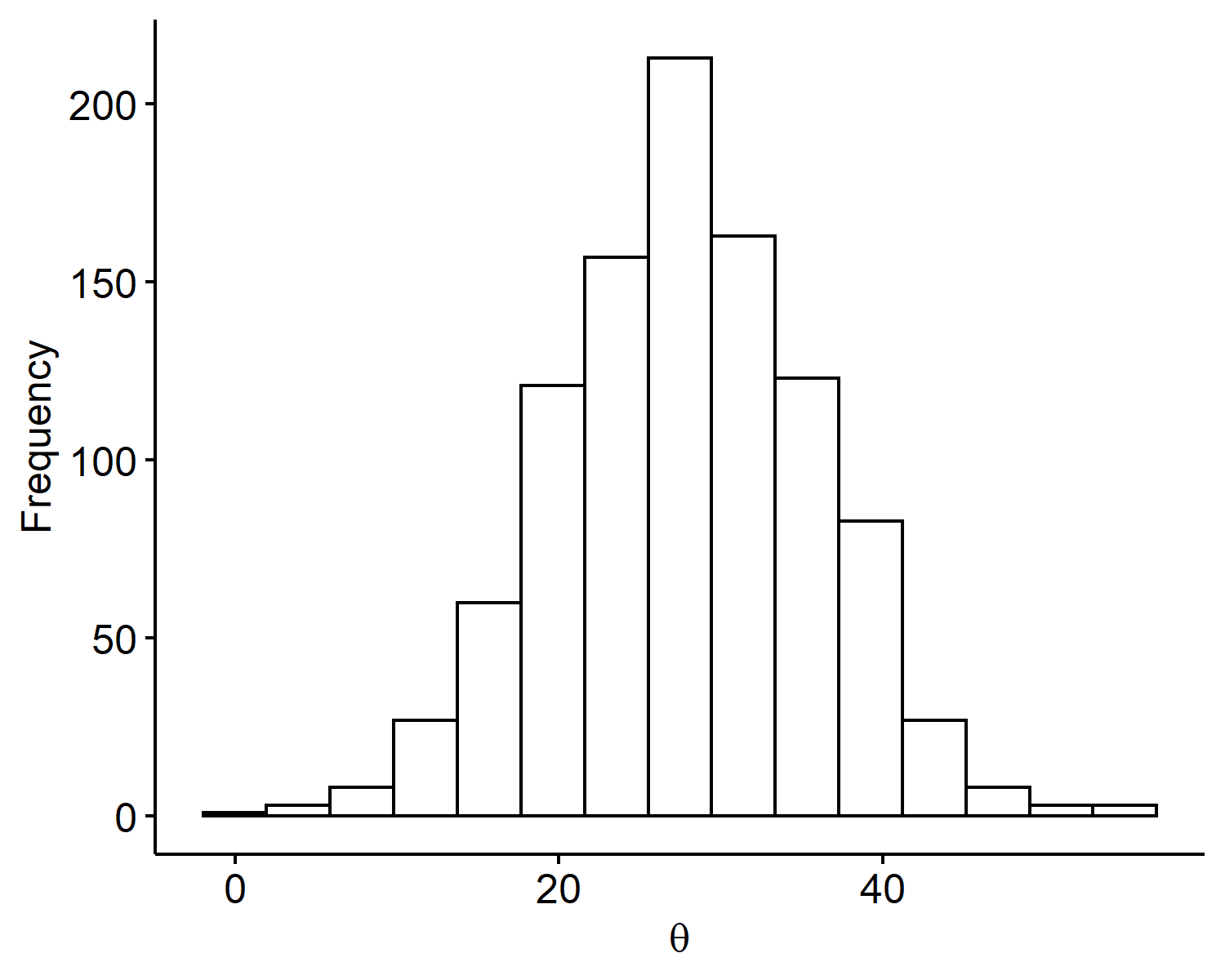
Thus the prior is set to be $\theta \sim N(28, 8^2)$. Note that prior information is very subjective, and it’s not always easy to interpret the hyperparameters. If we are, say, 99% confident, then we may go out 3 sd’s instead of 2. Ultimately because we have 200 data points, this shouldn’t affect our posterior too much as it’s dominated by the observed data. Below is a plot of $S=1000$ Monte Carlo samples from our prior distribution generated via:
Posterior and posterior summaries
Using the formula for $\mu_n$ and $\tau_n^2$, the posterior mean and variance are
The 95% credible interval for $\theta$ is (31.18mm, 33.06mm). Although we already know the true posterior distribution, we can use MC samples to find the mean and variance.
Posterior mean and variance decomposition
Just like in previous models, we can write the posterior mean for $\theta$ as a weighted average of the prior mean and sample mean. We can also find a similar decomposition for a quantity related to the posterior variance for $\theta$. The formulas are messy, and they become much easier to write in terms of the sampling and prior precisions:
Precision is just defined as the inverse of the variance. Whereas variance is interpreted as “degree of variability”, precision can be thought of as “amount of information”. With these quantities, the posterior mean decomposition is
With more observed data ($n \rightarrow \infty$), the posterior mean is dominated by the sample mean $\bar{y}$.
The posterior precision decomposition is:
This says the “posterior information” is equal to the prior information plus information from the data.
Posterior predictive checks
A common way to assess model fit is to perform a posterior predictive check. The idea is our posterior for $\theta$ represents our updated beliefs about the mean carapace length after observing data. If we appropriately modeled carapace lengths (by our normal model), then new predictions from our sampling model should look similar to our observed data.
Recall what our observed data look like in Figure 1. When we generate new predictions, we want to see the new values to be within 10 to 50, roughly symmetric, and center around 30.
The new predictions are generated from our sampling model, because the sampling model describes how our data is generated given parameters $\theta$ and $\sigma^2$.
Note that the tilde on $Y$ represents a new prediction. Since the posterior mean $E(\theta \mid y)$ represents the mean updated belief about $\theta$, we could plug its value (32.1mm) in and generate predictions from:
However, this method doesn’t account for the posterior uncertainty in $\theta$. A better way is to average over the posterior distribution of $\theta$ by computing the posterior predictive distribution:
Formally, the posterior predictive distribution can be difficult to compute in closed-form. However, it is much simple to sample from the posterior prediction distribution using Monte Carlo. The process is we first sample a $\theta$ from the posterior distribution, and then draw from the predictive model centered at $\theta$:
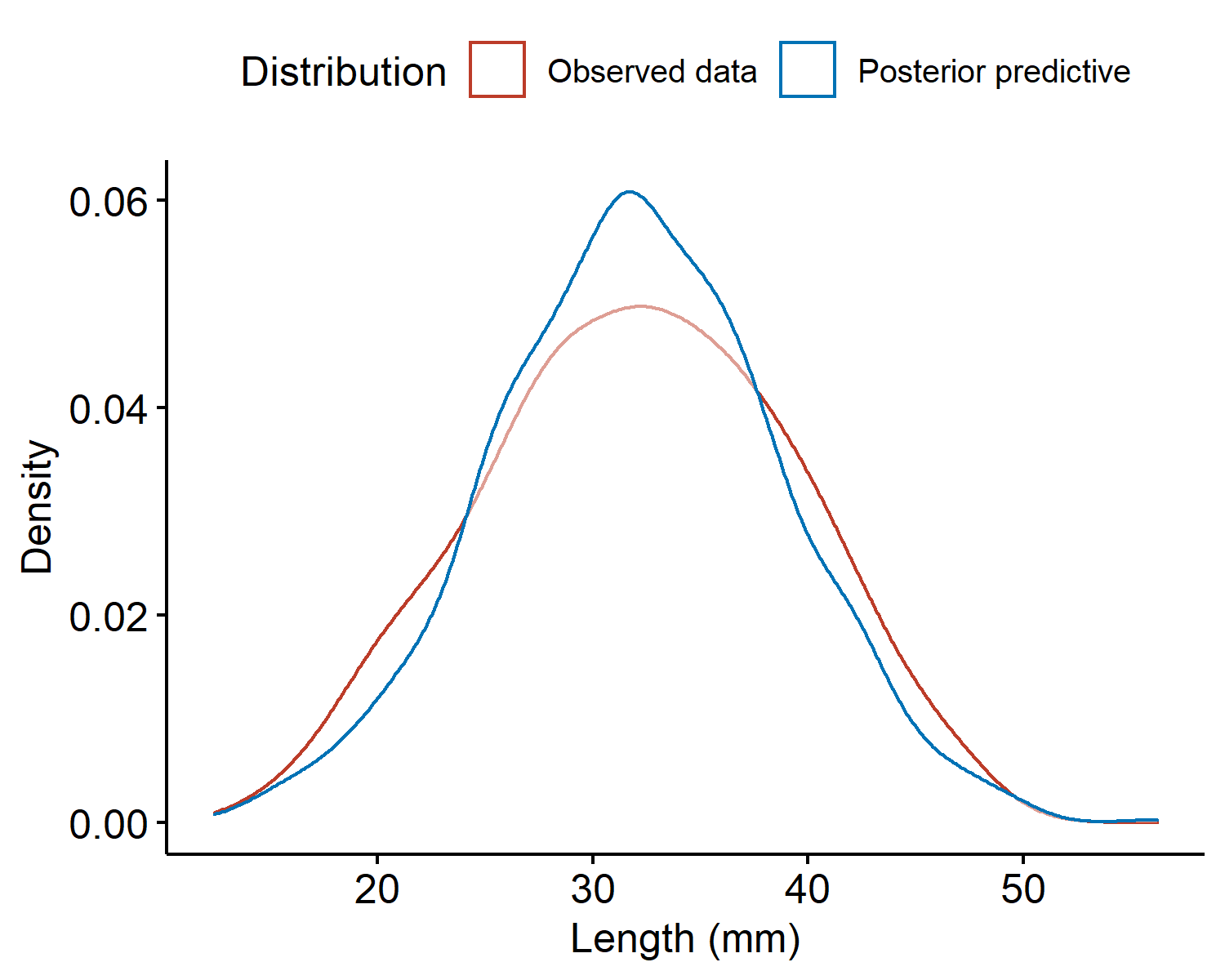
Then the set of values $\{\tilde{y}^{(1)}, \cdots, \tilde{y}^{(S)}\}$ is the empirical distribution of the posterior predictive. For our crab example, the densities of the observed data and the posterior predictive are given below.
| |
The two densities look similar and are centered around the same value. However, the observed data density has heavier tails (i.e. is more spread out) than the posterior predictive, indicating our sample model underestimated the variability $\sigma^2$. We might assume a larger value for $\sigma^2$ to better represent the variability in the data, or instead of fixing $\sigma^2$ we place a prior on both parameters and get a posterior distribution for both. This would allow the data to drive what the value should be.
Improper priors
One other issue that hasn’t arisen yet is known as an improper prior. Suppose we have the normal sampling model with unknown mean $\theta$ and known variance $\sigma^2$. What if we have no prior information about $\theta$?
A candidate prior model is:
where any real number is equally plausible. This prior model is not a valid distribution mathematically. However, using this expression as the prior results in a closed-form posterior which is a valid distribution!
Note that improper priors can result in model instability. For this particular model3, this prior works because we have a large amount of data. With a smaller dataset, suggesting such a large range of possible values of $\theta$ can make things messy. In general, we should be cautious when using them, and should use a valid prior distribution with large variance if possible.
Campbell, N.A. and Mahon, R.J., 1974. A multivariate study of variation in two species of rock crab of the genus Leptograpsus. Australian Journal of Zoology, 22(3), pp.417-425. ↩︎
R code for plotting:
↩︎1 2 3 4 5 6 7 8library(ggpubr) data(crabs, package = "MASS") mean(crabs$CL) var(crabs$CL) gghistogram(crabs, x = "CL", add_density = T, xlab = "Carapace length (mm)", ylab = "Frequency")The other place we might see improper priors is in linear regression. Often times we place improper priors on the regression coefficients. ↩︎
| Apr 26 | A Bayesian Perspective on Missing Data Imputation | 11 min read |
| Apr 19 | Bayesian Generalized Linear Models | 8 min read |
| Apr 12 | Penalized Linear Regression and Model Selection | 18 min read |
| Apr 05 | Bayesian Linear Regression | 18 min read |
| Mar 29 | Hierarchical Models | 18 min read |