Hierarchical Models

This is our first step to extending a lot of the things we’ve talked about to slightly more complicated models.

Motivating example

Here’s the R packages used throughout this page.

1
2
3
4

library(tidyverse)
library(ggpubr)
library(rjags)
library(MCMCvis)

The data set is adapted from Hoff’s book, and presents the weekly time (in hours) spent on homework for students sampled from eight different schools. Data for school 5 were modified for demonstration purposes.

 1
 2
 3
 4
 5
 6
 7
 8
 9
10
11
12
13
14
15
16
17
18
19

baseURL <- "http://www2.stat.duke.edu/~pdh10/FCBS/Exercises"
dat <- NULL
for (i in seq(8)) {
  if (i != 5) {
    dat <- bind_rows(
      dat,
      data.table::fread(str_glue("{baseURL}/school{i}.dat")) %>%
        mutate(school = i)
    )
  }
}

dat <- dat %>%
  select(school, hwtime = V1) %>%
  bind_rows(data.frame(
    school = 5,
    hwtime = c(12.97, 1.14, 15.08, 10.84, 14.21, 7.11, 13.19, 16.00, 17.47)
  )) %>%
  arrange(school, hwtime)

Exploratory data analysis

A summary of the data by school can be found in the table below.

First thing to note is that the sample sizes are all around 20 except for school 5, which only has 9 students. The average time spent is also higher, which might be an artifact solely due to the smaller sample size, or it could be evidence that students from school 5 spend more time on their homework than their peers.

1
2
3

ggboxplot(dat, x = "school", y = "hwtime",
          color = "school", palette = "nejm",
          xlab = "School", ylab = "Hours spent")

Figure 1: Boxplot of weekly time spent on homework by school.

The rest of the schools seem roughly similar to each other, although school 1 seems to have a slightly higher mean. Maybe we trust this more because of school 1’s larger sample size.

Our goal is to estimate the average weekly time spent on homework across the country, while also identifying schools within this particular data set that stand out. Let \(J\) denote the number of groups (schools), \(n_j\) be the number of observations within group \(j\), and \(n = \sum_{j=1}^J n_j\) be the overall total number of observations. Obviously we have \(J=8\) and \(n = 165\).

We will sequentially go through three different modeling strategies for this data set, where the first two are going to be things we’ve dealt with in the past. Soon we’ll see why these models aren’t very suitable for this structure of data.

Model 1 – complete pooling

Let \(Y_{ij}\) be the amount of time spent on homework for student \(i\) from school \(j\), for \(i = 1, \cdots, n_j\) and \(j = 1, \cdots, J\). Our first sampling model is:

We’re specifying it this way because the observations are continuous values. We are assuming all observations, regardless of which school they came from, are from the same distribution. With conditional independence, the sampling density function is:

For our prior model, we are going to assume fairly little intuition¹ about the parameters. We will specify:

Posterior samples via JAGS

Using JAGS, we may obtain the following posterior sample densities and trace plots.

 1
 2
 3
 4
 5
 6
 7
 8
 9
10
11
12
13
14
15
16
17
18
19
20
21
22
23
24
25
26
27
28
29
30
31
32
33
34
35
36
37
38
39
40
41
42
43
44
45
46
47
48
49
50
51
52
53
54
55
56
57
58
59
60
61
62
63
64
65
66
67
68
69
70
71

# (1) Specify sample size n and create a data list
n <- nrow(dat)
dataList1 <- list(
  "hwtime" = dat$hwtime,
  "n" = n
)

# (2) Specify list of parameter(s) to be monitored
params1 <- c("theta", "sig2")

# (3) Specify initial values for parameters in Metropolis-Hastings algorithm
y_bar <- mean(dat$hwtime)
s <- sd(dat$hwtime)

initsValues <- list(
  "theta" = y_bar,
  "inv_sig2" = 1 / s^2
)

# (4) Specify parameters for running Metropolis-Hastings algorithm
adaptSteps <- 10000     # steps to "tune" the samplers
burnInSteps <- 20000    # steps to "burn-in" the samplers
nChains <- 3            # chains to run
numSavedSteps <- 50000  # total steps in chains to save
thinSteps <- 10         # steps to "thin" (1 = keep every step)
nIter <- ceiling((numSavedSteps*thinSteps)/nChains)  # steps / chain

# (5) Create, initialize, and adapt the model
set.seed(42)
model1 <- textConnection("
model
{
  # Sampling model - in JAGS, the first argument for the normal distribution
  # is the mean theta, while the second is the precision = 1/sigma^2
  for (i in 1:n) {
    hwtime[i] ~ dnorm(theta, inv_sig2)
  }

  # Prior model for theta and inv_sig2
  # Note that we specify sig2 ~ IG(0.01,0.01), which is equivalent to the
  # precision inv_sig2 ~ Gamma(0.01,0.01)
  theta ~ dnorm(20, 1/(10^2))
  inv_sig2 ~ dgamma(0.01, 0.01)

  # Parameter transformation
  # We specify our prior on the precision inv_sig2 because JAGS does not have
  # inverse-gamma distributions built in; however, we want the posterior dist
  # ultimately for the variance, computed by sig2 = 1/inv_sig2
  sig2 <- 1/inv_sig2
}
")
jagsModel1 <- jags.model(model1,
                         data = dataList1,
                         inits = initsValues,
                         n.chains = nChains,
                         n.adapt = adaptSteps)
close(model1)

# (6) Burn-in the algorithm
if (burnInSteps > 0) {
  update(jagsModel1, n.iter = burnInSteps)
}

# (7) Run MCMC algorithm
codaSamples1 <- coda.samples(jagsModel1,
                             variable.names = params1,
                             n.iter = nIter,
                             thin = thinSteps)

# (8) Diagnose convergence and plot posterior densities
plot(codaSamples1)

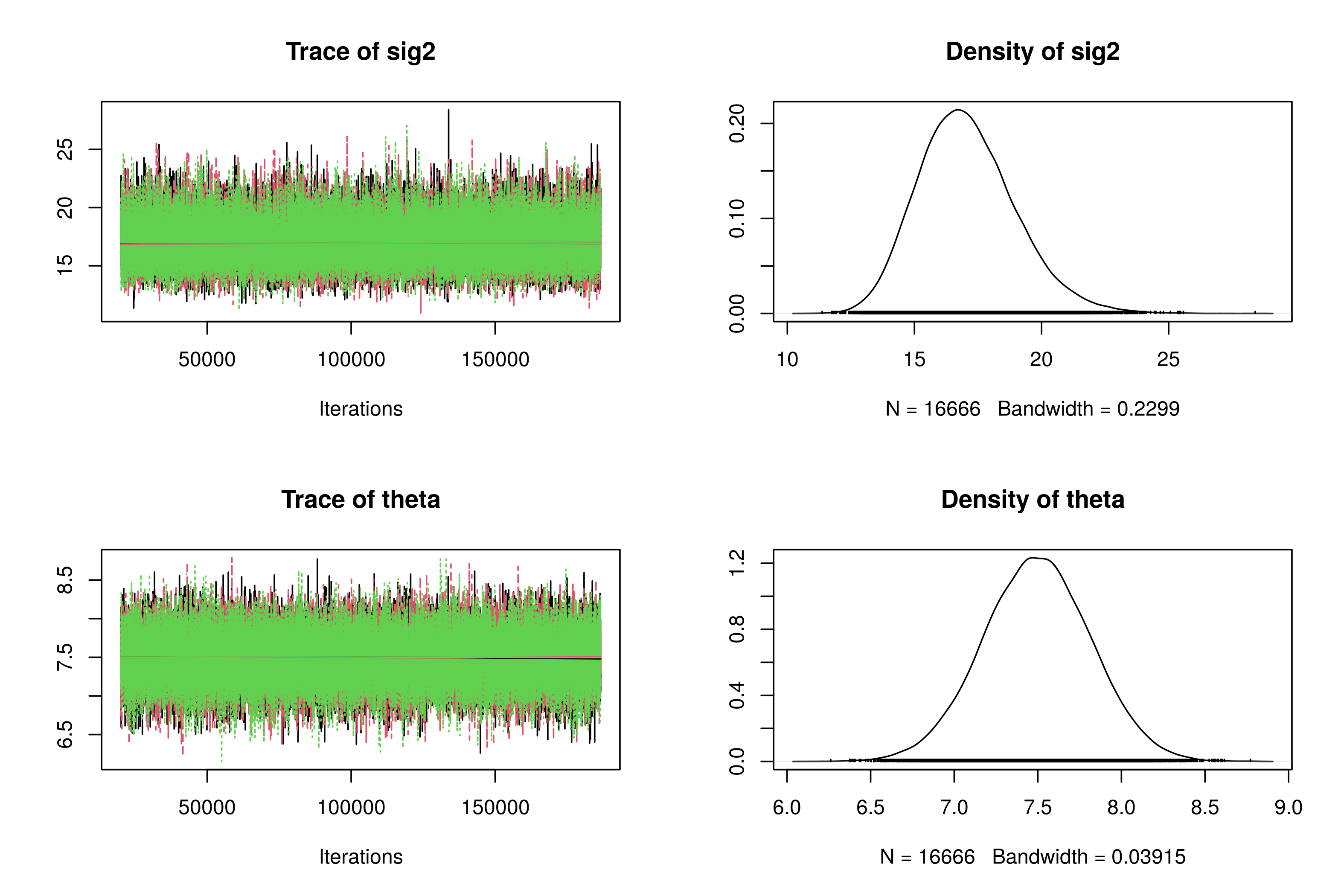
Figure 2: Trace plots and posterior densities for Model 1.

Both trace plots indicate convergence because the chains are oscillating among the same set of values. The posterior median for \(\sigma^2\) is about 16.95, and the posterior mean for \(\theta\) is about 7.49.

Issues

The primary issue here is that we cared about comparing the schools, but the way we specified this model, i.e. aggregating all schools into one model, doesn’t incorporate the information about the schools at all!

The “complete pooling” in the name of this model is a reference to t-tests – in some cases we pool the samples together and estimate the variance based on the combined sample. It’s essentially the same idea here where we pool all the samples together into one big data set, and only estimate one set of parameters.

Model 2 – no pooling

We can address the issue in Model 1 by writing down a model which accounts for the group structure. An alternative way to specify the sampling model is to specify a separate model for each of the schools. Within group \(j\),

We are giving each school its own \(\theta_j\) and \(\sigma_j^2\) because we may want to estimate the average and variance for each school. Assuming conditional independence across all \(J\) groups, the density for all our data is given by:

In this model we have a total of 16 parameters to estimate:

\begin{gathered} \boldsymbol{\theta} = (\theta_1, \cdots, \theta_J)' \\ \boldsymbol{\sigma}^2 = (\sigma_1^2, \cdots, \sigma_J^2)' \end{gathered}

We will specify the same prior model for all the parameters. Assuming independence across all \(J\) groups:

Since we specified independence between groups, we can essentially fit each group’s model separately!

Posterior samples

We may generate posterior samples using JAGS in a similar fashion. Viewing eight sets of trace plots and posterior densities can be cumbersome, so we use boxplots instead to summarize our posterior samples.

 1
 2
 3
 4
 5
 6
 7
 8
 9
10
11
12
13
14
15
16
17
18
19
20
21
22
23
24
25
26
27
28
29
30
31
32
33
34
35
36
37
38
39
40
41
42
43
44
45
46
47
48
49
50
51
52
53
54
55
56
57
58
59
60
61
62
63
64
65
66
67
68
69
70
71
72
73

# Data list
J <- length(unique(dat$school))

dataList2 <- list(
  "hwtime" = dat$hwtime,
  "school" = dat$school,
  "n" = n,
  "J" = J
)

# Parameters of interest to be monitored
params2 <- c("theta", "sig2")

# Initial values
initsValues2 <- list(
  "theta" = rep(y_bar, J),
  "inv_sig2" = rep(1/s^2, J)
)

# Specify model
model2 <- textConnection("
model
{
  # Sampling model
  # Note that each hwtime value comes from a normal distribution with mean and
  # precision parameters corresponding to the school the student belongs to!
  for (i in 1:n) {
	  hwtime[i] ~ dnorm(theta[school[i]], inv_sig2[school[i]])
  }

  # Prior model for theta[j] and inv_sig2[j]
  for (j in 1:J) {
  	theta[j] ~ dnorm(20, 1/(10^2))
	  inv_sig2[j] ~ dgamma(0.01, 0.01)

  	# Parameter transformation (just like in Model 1)
	  # Need to have model calculate sig2[j] = 1/inv_sig2[j]
	  sig2[j] <- 1/inv_sig2[j]
  }
}
")

jagsModel2 <- jags.model(model2,
                         data = dataList2,
                         inits = initsValues2,
                         n.chains = nChains,
                         n.adapt = adaptSteps)

close(model2)

# Run MCMC
set.seed(42)
if (burnInSteps > 0) {
  update(jagsModel2, n.iter = burnInSteps)
}

codaSamples2 <- coda.samples(jagsModel2,
                             variable.names = params2,
                             n.iter = nIter,
                             thin = thinSteps)

map2_dfr(codaSamples2, seq(nChains),
  ~ .x %>%
    as.data.frame() %>%
    mutate(Chain = .y) %>%
    pivot_longer(-Chain, names_to = "Parameter", values_to = "Value")
) %>%
  mutate(
    School = str_replace(Parameter, ".*\\[(\\d)\\]$", "\\1"),
    Parameter = str_remove(Parameter, "\\[\\d\\]$")
    ) %>%
  filter(Parameter == "theta") %>%
  ggboxplot(x = "School", y = "Value")

From the posterior samples of \((\theta_1, \cdots, \theta_8)\), we can see that school 5 still looks higher than other schools, but there is also more variability due to the smaller sample size.

Caterpillar plots

We can do the same thing for \(\sigma^2\), or we may take advantage of the MCMCvis R package. In what’s called caterpillar plots below, points are medians, thin lines are 50% credible intervals, and thick lines are 95% credible intervals.

1
2
3
4
5

par(mar = c(2, 1, 2, 1), mfrow = c(1, 2))
MCMCplot(codaSamples2, params = "theta",
         main = "Posterior CIs for theta", ref = y_bar)
MCMCplot(codaSamples2, params = "sig2",
         main = "Posterior CIs for sigma2", ref = s^2)

Figure 3: Catepillar plots of `\(\theta\)` and `\(\sigma^2\)`.

We may then use these CIs to compare between groups². For example, the 95% CIs for \(\theta_5\) and \(\theta_6\) don’t overlap, indicating evidence that school 5 students average more time on homework per week.

Issues

Suppose we knew the true mean time studying per week for schools 1-7, i.e. \(\theta_1, \cdots, \theta_7\). Does that tell us information about \(\theta_8\)? Well, possibly, as we might expect \(\theta_8\) to be similar to values for \(\theta_1, \cdots, \theta_7\) if schools were somewhat related. This dependence across groups violates our between-group independence assumption.

The other issue is that this model does not inform us about the true overall mean time \(\mu\), regardless of the school. How could we “combine” estimates of \(\theta_1, \cdots, \theta_8\) to get a posterior for \(\mu\)? Simply taking the average of the eight values might give us a crude guess, but it doesn’t make sense to give all \(\theta\)’s the same weight as the sample sizes could be different. It makes more sense to build \(\mu\) into our model.

We named this model “no pooling” because we are not grouping any observations together unless they are from the same school. We are not combining information across groups.

Model 3 – hierarchical

Our next step is to address the issues posed in Model 2. More specifically, how can we account for the fact that our group means are likely to be related to each other?

Sampling and prior distributions

Let assume the variances within each group are unknown but equal, i.e. \(\sigma_j^2 = \sigma^2\) for all \(j\). Then we will specify the sampling model in two pieces. The within-group sampling model looks very similar to the one in Model 2. For group \(j\),

We still assume conditional independence across groups:

Now comes the second part where we account for the possible dependency between the \(\theta\)’s, the between-group sampling model. Since we believe the group means are related, we model them as values drawn from a between-group model:

Here \(\mu\) can be interpreted as the “overall mean” across all groups, and \(\tau^2\) is the between-group variance. This describes heterogeneity across group means. We also assume conditional i.i.d. here, so

The \(\theta\)’s are conditionally independent although they all come from the same distribution that’s centered at \(\mu\). This is going to have an interesting effect on the estimates that we get for those school averages.

Now that we have specified distributions for the \(Y\)’s and the \(\theta\)’s, there are still three parameters that we don’t have distributions for – \(\mu\), \(\tau\), and \(\sigma^2\).

The prior for \(\mu\) is the same as the one we used for the \(\theta_j\)’s before as we no longer need to specify priors for the \(\theta_j\)’s. We could specify inverse gamma priors for \(\tau\) and \(\sigma\), but we don’t have to anymore because conjugacy is not required for JAGS³. 1000 was chosen as an arbitrary upper bound for the standard deviations, which shouldn’t matter too much as long as the value is “large enough”. Inverse-gamma priors such as \(\text{IG}(0.01, 0.01)\) for variance parameters are notoriously poor and sensitive if the true variance is close to 0 (see Gelman, 2006). This is more important of an issue typically when estimating the bwteen-group variance \(\tau^2\).

Putting everything together, our model looks like the following. This is called a hierarchical model because there’s multiple layers to the (sampling) model, in particular the within-group model, the between-group level, and the prior model on the top layer.

Posterior samples

Using JAGS, we may obtain posterior samples and inspect the posterior CIs for the parameters.

 1
 2
 3
 4
 5
 6
 7
 8
 9
10
11
12
13
14
15
16
17
18
19
20
21
22
23
24
25
26
27
28
29
30
31
32
33
34
35
36
37
38
39
40
41
42
43
44
45
46
47
48
49
50
51
52
53
54
55
56
57
58
59
60
61
62
63
64
65
66
67
68
69
70

dataList3 <- list(
  "hwtime" = dat$hwtime,
  "school" = dat$school,
  "n" = n,
  "J" = J
)

params3 <- c("theta", "mu", "sig2", "tau2")

initsValues3 <- list(
  "theta" = rep(y_bar, J),
  "mu" = y_bar,
  "sig" = s,
  "tau" = 1
)

model3 <- textConnection("
model
{
  # Sampling model - in JAGS, the first argument for the normal distribution
  # is the mean theta[j], while the second is the precision = 1/sigma^2
  # Within-group model
  for (i in 1:n) {
	hwtime[i] ~ dnorm(theta[school[i]], inv_sig2)
  }

  # Between-group model
  for (j in 1:J) {
  	theta[j] ~ dnorm(mu, inv_tau2)
  }

  # Prior model for mu, sig, and tau
  mu ~ dnorm(20, 1/(10^2))
  sig ~ dunif(0, 1000)
  tau ~ dunif(0, 1000)

  # Parameter transformation
  # This computes the precision, e.g., inv_sig2 = sig^(-2)
  inv_sig2 <- pow(sig, -2)
  inv_tau2 <- pow(tau, -2)

  # Since we most likely care about the posterior samples of
  # variances, we can compute these here
  sig2 <- sig^2
  tau2 <- tau^2
}
")

jagsModel3 <- jags.model(model3,
                         data = dataList3,
                         inits = initsValues3,
                         n.chains = nChains,
                         n.adapt = adaptSteps)
close(model3)

set.seed(42)
if (burnInSteps > 0) {
  update(jagsModel3, n.iter = burnInSteps)
}

codaSamples3 <- coda.samples(jagsModel3,
                             variable.names = params3,
                             n.iter = nIter,
                             thin = thinSteps)

par(mar = c(2, 1, 2, 1), mfrow = c(1, 2))
MCMCplot(codaSamples3, params = c("theta", "mu"), ref = NULL,
         main = "Posterior CIs for mean parameters")
MCMCplot(codaSamples3, params = c("sig2", "tau2"), ref = NULL,
         main = "Posterior CIs for variance parameters")

Figure 4: Posterior CIs for the parameters of interest.

On the left we have the 50% and 95% credible intervals for \((\theta_1, \cdots, \theta_8)\) and \(\mu\). We can still see \(\theta_5\) to be above the other groups in terms of group means. We also get an overall mean estimate, which is a benefit that we didn’t have in Model 2.

On the right we have the posterior CIs for the variance parameters \(\sigma^2\) and \(\tau^2\). The within-group variance is considerably larger than the between-group variance, which is evidence that there’s not an effect associated with the particular grouping variable.

Benefits of hierarchical models

Model 3 is known as a hierarchical or multi-level model because it is characterized by multiple layers within the model to represent natural group structure⁴. Hierarchical modeling is a major strength of Bayesian inference due to:

• the intuitive interpretation associated with writing the model down,
• the ability to generate posterior samples via computational methods, and
• classical frequency estimation procedures are difficult to apply to complex hierarchical models.

Hierarchical models are a natural compromise between two extreme models: complete pooling where parameters are estimated assuming all data come from the same population, and no pooling where parameters for each group are estimated completely independently of any other group. In model 3, we see partial pooling of our estimates, meaning that information can be borrowed across groups to help with estimation.

Recall that school 5 has a very small sample size (\(n_5 = 9\)). This partial pooling is useful because we can “borrow” information from other groups to assist in estimating \(\theta_5\).

Shrinkage

In conjunction with this point, posterior estimates of the group means \(\theta_j\) exhibit a property called shrinkage, which is a common phenomenon in statistics. For example, traditional linear regression methods can break down when there’s a large number of features (covariates) relative to the sample size. Penalized regression methods such as ridge regression and Lasso regression impose constraints on the regression coefficients to overcome this issue, and the effect is pushing regression coefficients towards zero.

The same pattern shows up with the hierarchical models. When comparing the posterior mean estimates for \((\theta_1, \cdots, \theta_8)\) in models 2 and 3, estimated \(\theta_5\) values are considerably different.

To observe this effect more clearly, we may use a scatter plot for the posterior estimates in the two models. The posterior mean for \(\mu\) from model 3 was 7.77, as shown by the dashed line.

Figure 5: Posterior estimates of within-group mean parameters.

In some cases, e.g. schools 2, 4 and 8, there’s not that much of a difference between the two model estimates. However, there is a large difference with the \(\theta_5\) estimates. Because we had a small sample size, the model essentially “trusts” the data within that group less, and shrinks \(\theta_5\)’s estimate towards \(\mu\), i.e. borrowing information from the other groups. Model 3 pushes group-level estimates from Model 2 closer to \(\mu\).

In summary, with hierarchical models, shrinkage allows estimates of group means to shrink towards the overall mean. The degree to which a group’s estimate shrinks depends on its sample size and within-group variation. Estimates for groups with larger sample sizes are generally more precise.

Shrinkage is a natural property arising within Bayesian hierarchical models, but hs also been explored in the frequentist literature. To learn more, search for shrinkage estimators such as the James-Stein estimator.

Multiple comparisons

Finally, hierarchical modeling can help to automatically alleviate issues arising with adjusting for multiple comparisons. Notice from Figure 4 that Model 2 might imply the true mean for school 5 is different from school 6 since their 95% CIs don’t overlap. If we did more comparisons between \(\theta_5\) and \(\theta_4, \theta_6, \theta_7\), we might say school 5 students average more time on homework than schools 4, 6 and 7.

However, if we look at Model 3, we no longer get the same conclusion because the credible intervals overlap. There’s not enough evidence to suggest a significant difference between \(\theta_5\) and \(\theta_4, \theta_6, \theta_7\).

Figure 6: Posterior CIs for mean parameters in Model 3.

Final notes

In Model 3, we assumed all groups have the same unknown variance \(\sigma^2\). We could extend this and let each group to have its own unknown variance \(\sigma_j^2\), but it’s not common in practice since most interest is on inference of the mean parameters, and we essentially need more samples because the variance is harder to estimate.

If we had chosen inverse-gamma priors for both variance parameters in Model 3, we can use a Gibbs sampler as all of the full conditionals can be derived explicitly. It’s highly efficient compared to Metropolis-Hastings, but not necessarily the best modeling choice.

Finally, Model 3 is the Bayesian analog of a random effects or variance components model in the frequentist setting. The schools are a random sample from a collection of a large population of schools. We do care about the group-specific effects (school averages), but we also care about comparing the effects of the schools in general and the average of all schools. Hierarchical models can also have more than two levels!