Seasonal Time Series
In the last chapter, we learned about how to deal with mean and variance changes in time series data. Periodic patterns are also frequently observed, and we will use seasonal ARIMA models for this type of data.
Motivating example
The data are the monthly sales of six types of wines Australian wines (red, rose, sweet white, dry white, sparkling, and fortified) for years 1980-1994. The units are thousands of liters. We’ll focus on the red wine sales data, and use the ts() function to turn the column into a time series object.
| |
As always, we first plot the series and its ACF and PACF. On top of the mean and variance increases over time, we also observe a periodical pattern that repeats every year. This means we might be able to use the sales in June 1985 to predict the sales in June 1986. In seasonal AR(1) (MA(1)), $X_{t-12}$ ($Z_{t-12}$) can be used to predict $X_t$; in seasonal AR(2), $X_{t-12}$ and $X_{t-24}$ can be used to predict $X_t$, etc.
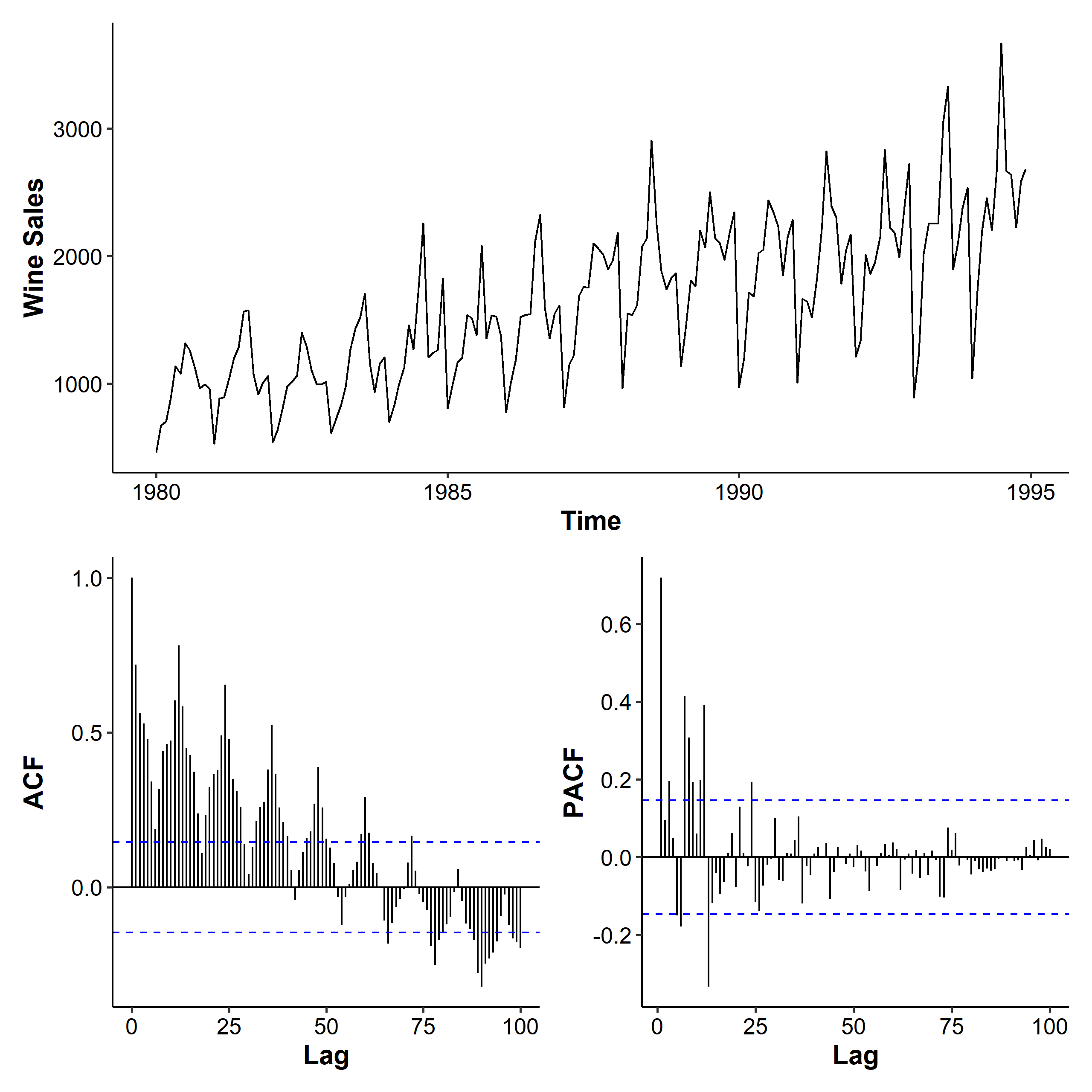
When we see a seasonal pattern in the time series plot, it’s often desirable to increase the lag.max parameter when plotting the ACF and PACF to see the entire pattern. The ACF slowly decreases as a result of the series being trended. Because the series is seasonal, the ACF for the seasonal lags (12, 24, 36, etc. multiples of the seasonal frequency) are higher than the ACF of the other lags. We see a combination of these effects for this trended, seasonal data.
This effect could be removed using seasonal differencing. But before that, let’s see some simpler models first.
Seasonal ARMA
A seasonal pattern occurs when a time series is affected by seasonal factors such as the time of the year or the day of the week. Seasonality is always of a fixed and known period.
The frequency is the number of observations before the seasonal pattern repeats1.
Seasonal MA(1)
We will start with the seasonal MA(1) model. As we have monthly data in the motivating example, let’s say the period $s=12$. The $MA(1)_{s=12}$ model is
$$ X_t = \mu + Z_t + \Theta Z_{t-12}, \quad Z_t \overset{i.i.d.}{\sim} WN(0, \sigma^2) $$
Recall that the MA(1) model had a linear combination of $Z_t$ and $Z_{t-1}$, but in our seasonal MA(1) model we have a combination of $Z_t$ and $Z_{t-12}$ where the 12 corresponds to the period. If we didn’t know there’s a seasonal pattern, we could call this an MA(12) model. The $\Theta$ notation is to emphasize the seasonality.
Calculating the ACF is similar to the process for the MA(1) model. We first find the autocovariance function:
$$ \begin{aligned} \gamma_X(0) &= Var(X_t) = Var(Z_t) + \Theta^2 Var(Z_{t-12}) + 0 \\ &= (1 + \Theta^2)\sigma^2 \\ \gamma_X(k) &= Cov(X_t, X_{t-k}), \quad k \geq 1 \\ &= Cov(Z_t + \Theta Z_{t-12}, X_{t-k}) \\ &= \underbrace{Cov(Z_t, X_{t-k})}{=0} + \Theta Cov(Z{t-12}, X_{t-k}) \\ &= \Theta Cov(Z_{t-12}, Z_{t-k} + \Theta Z_{t-12-k}) \\ &= \Theta Cov(Z_{t-12}, Z_{t-k}) + \Theta^2 \underbrace{Cov(Z_{t-12}, Z_{t-12-k})}_{=0} \\ &= \begin{cases} \Theta \sigma^2, & k = 12 \\ 0, & \text{otherwise} \end{cases} \end{aligned} $$
Thus the ACF is
$$ \rho_X(k) = \begin{cases} \frac{\Theta}{1 + \Theta^2}, & k = 12 \\ 0, & \text{otherwise} \end{cases} $$
To find the theoretical ACF, we may use the ARMAacf() function in R. The theoretical PACF can be found by setting parameter pacf = TRUE. We can see that all ACF values are zeros except at $k=12$. For the PACF, there are spikes at lags that are multiples of 12.
| |
Seasonal MA(Q)
In general the $MA(Q)_s$ model is
$$ X_t = Z_t + \Theta_1 Z_{t-s} + \Theta_2 Z_{t-2s} + \cdots + \Theta_Q Z_{t-Qs}, \quad Z_t \overset{i.i.d.}{\sim} WN(0, \sigma^2) $$
The ACF has spikes at lags $s, 2s, \cdots, Qs$ and is zero afterwards. The PACF exponentially decreases at lags that are multiples of $s$ and is zero for other lags.
Seasonal AR(1)
The $AR(1)_{12}$ model is
$$ X_t = \Phi X_{t-12} + Z_t, \quad Z_t \sim WN(0, \sigma^2) $$
Again, this is similar to the AR(1) model with the $X_{t-1}$ term replaced by $X_{t-12}$. The ACF is
$$ \rho_X(12k) = \Phi^k, \quad k = 0, 1, 2, \cdots $$
which is found from
$$ \begin{aligned} \gamma_X(0) &= \frac{\sigma^2}{1 - \Phi^2} \\ \gamma_X(k) &= \begin{cases} \frac{\sigma^2\Phi^k}{1 - \Phi^2}, & k = 12, 24, 36, \cdots \\ 0, & \text{otherwise} \end{cases} \end{aligned} $$
Seasonal AR(P)
The $AR(P)_s$ model is
$$ X_t = \Phi_1 X_{t-s} + \Phi_2 X_{t-2s} + \cdots + \Phi_P X_{t-Ps} + Z_t, \quad Z_t \sim WN(0, \sigma^2) $$
The ACF exponentially decreases at lags that are multiples of $s$. The PACF spikes at lags that are multiples of $s$ and takes value zero for all other lags.
Seasonal ARMA(1, 1)
The $ARMA(1, 1)_{12}$ model is
$$ X_t = \Phi X_{t-12} + Z_t - \Theta Z_{t-12}, \quad Z_t \sim WN(0, \sigma^2) $$
Alternatively, we can write it using the backshift operator:
$$ (1 - \Phi B^{12})X_t = (1 - \Theta B^{12})Z_t $$
The conditions for stationarity and invertibility are the same as the ones in the regular ARMA model: the absolute values of the roots of the characteristic equations should be larger than 1.
$$ \begin{gathered} \text{Stationarity: } |\Phi| > 1 \\ \text{Invertibility: } |\Theta| > 1 \end{gathered} $$
Multiplicative seasonal ARMA
Now we are going to combine the regular ARMA and seasonal ARMA models. This is done by multiplying the AR/MA polynomials. For example, the multiplicative combination of $MA(1)$ and $MA(1)_{12}$ is denoted $ARMA(0, 1) \times (0, 1)_{s=12}$, and can be expressed as
$$ X_t = (1 + \theta B)(1 + \Theta B^{12})Z_t = Z_t + \theta Z_{t-1} + \Theta Z_{t-12} + \theta\Theta Z_{t-13} $$
It’s not hard to show that $\gamma(0) = (1 + \theta^2)(1 + \Theta^2)\sigma^2$. We can also show that the ACF would have spikes at not only lags 1 and 12, but also 11 and 13.
$$ \begin{gathered} \rho(1) = \frac{\theta}{1 + \theta^2}, \quad \rho(12) = \frac{\Theta}{1 + \Theta^2}, \\ \rho(11) = \rho(13) = \frac{\theta\Theta}{(1 + \theta^2)(1 + \Theta^2)} \end{gathered} $$
The general form of an $ARMA(p, q) \times (P, Q)_s$ model is
$$ \Phi(B)\phi(B)X_t = \Theta(B)\theta(B)Z_t, \quad Z_t \overset{i.i.d.}{\sim}WN(0, \sigma^2) $$
where
$$ \begin{gathered} \phi(x) = 1 - \phi_1 x - \phi_x x^2 - \cdots - \phi_p x^p, \\ \Phi(x) = 1 - \Phi_1 x^s - \Phi_x x^{2s} - \cdots - \Phi_P x^{Ps}, \\ \theta(x) = 1 + \theta_1 x + \theta_2 x^2 + \cdots + \theta_q x^q, \\ \Theta(x) = 1 + \Theta_1 x^s + \Theta_2 x^{2s} + \cdots + \Theta_Q x^{Qs} \\ \end{gathered} $$
Here the AR order is $p + Ps$, the MA order is $q + Qs$, and the number of parameters is $p + P + q + Q$. We can also include an intercept term and add one to the total number of parameters. The order of the seasonal part of the model rarely goes higher than 1, especially after we include differencing.
For example, $ARMA(1, 0) \times (0, 2)_{12}$ can be written as
$$ (1 - \phi B) X_t = (1 + \Theta_1 B^{12} + \Theta_2 B^{24}) Z_t, $$
and the following model
$$ X_t = 0.6 X_{t-12} + Z_t + 0.4 Z_{t-1} - 0.8 Z_{t-12} - 0.32 Z_{t-13} $$
is $ARMA(0, 1) \times (1, 1)_{12}$.
ACF and PACF
In this section we’re going to explore the theoretical ACF and PACF of multiplicative seasonal ARMA models of different orders2. Just like how the (P)ACF of ARMA models were combinations of the (P)ACF of AR and MA models, we can think of multiplicative seasonal ARMA models as overlaying another seasonal component on the (P)ACF.
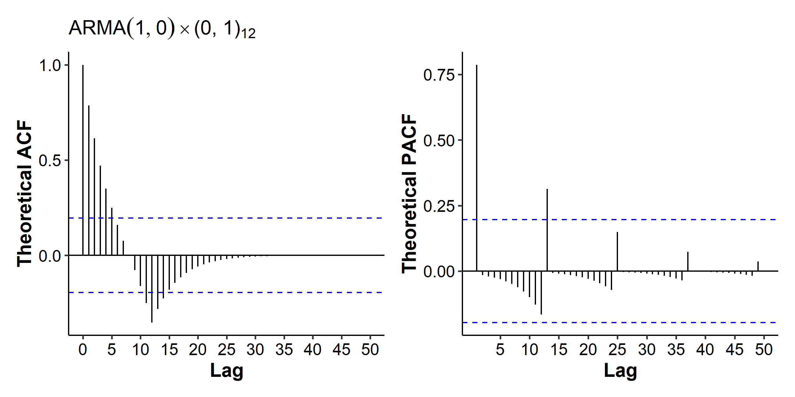
Starting with $ARMA(1, 0) \times (0, 1)_{12}$, we can use the following code to find its theoretical ACF and PACF:
| |
We look at the seasonal component first. In the ACF we see a spike at lag 12, and in the PACF we see spikes at lags that are multiples of 12. For the regular ARMA component, recall that for an AR(1) model, the ACF exponentially decays and the PACF should be cut off after lag 1. As a result, our ACF exponentially decays within each period, and the PACF has spikes at lags 1, 13, 25, 36 etc.
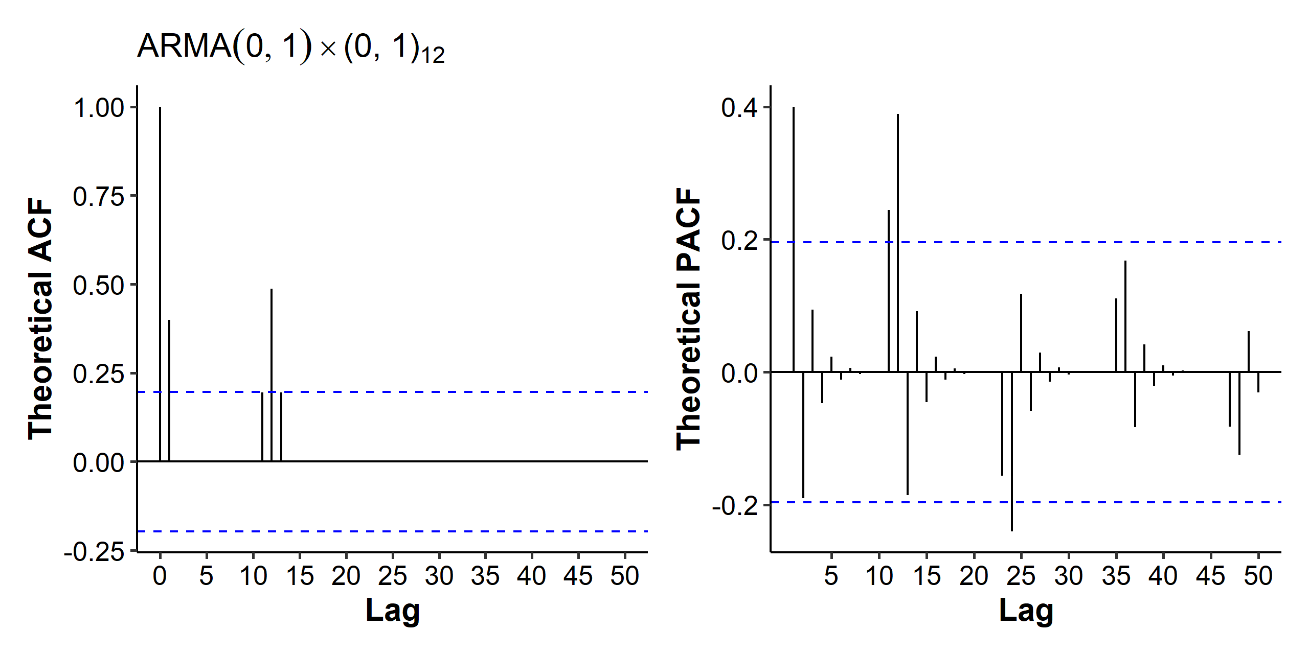
Next up we have an $ARMA(0, 1) \times (0, 1)_{12}$ model. For the seasonal component, again we see a spike at lag 12 in the ACF and tailing-off spikes at multiples of 12 in the PACF. The regular MA(1) model generates the spikes at lags 1, 11 and 13 for the ACF, and tailing off patterns between the periods for the PACF.
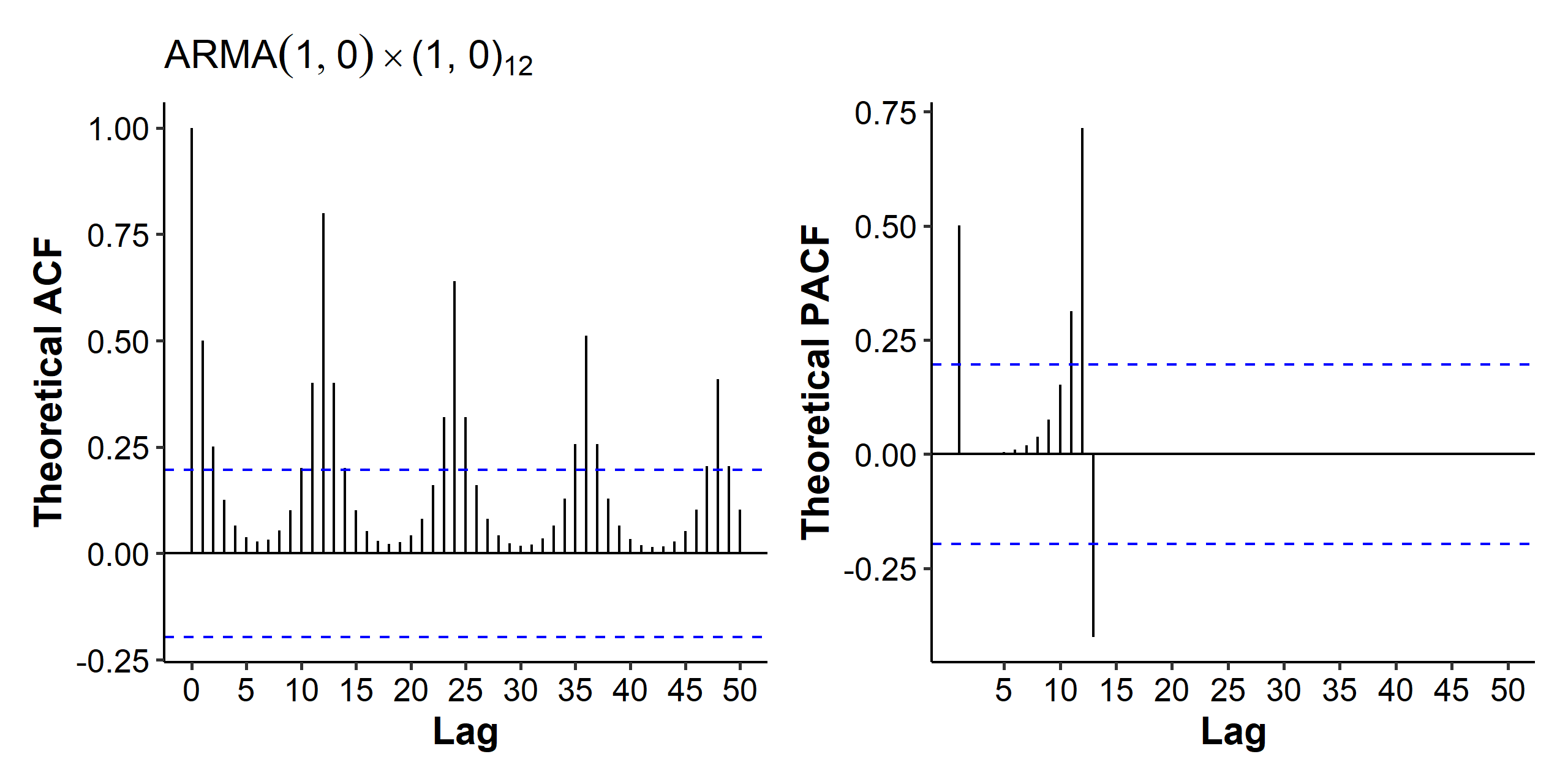
In the third example we have an $ARMA(1, 0) \times (1, 0)_{12}$ model:
$$ (1 - \Phi B^{12})(1 - \phi B)X_t = Z_t $$
where $\phi = 0.5$ and $\Phi = 0.8$. In the ARMAacf() function the coefficients are given as ar = c(0.5, rep(0, 10), 0.8, -0.5 * 0.8). With the seasonal AR(1) component, we see a tail off pattern at multiples of 12 in the ACF, and a spike at lag 12 in the PACF. The regular AR(1) contributes to the tail off pattern between the periods in the ACF, and the spikes at lags 1 and 13 in the PACF.
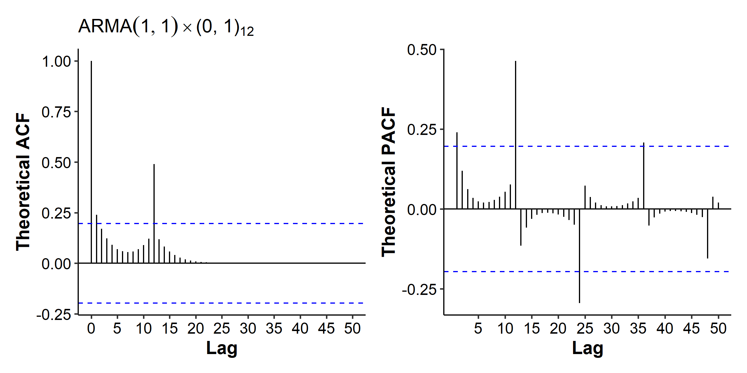
The last example is $ARIMA(1, 1) \times (0, 1)_{12}$. The MA(1) seasonal component gives us the spike at lag 12 in the ACF, and the tailing off spikes at multiples of 12 in the PACF. The regular ARMA(1, 1) generates the tailing off patterns between periods in both plots.
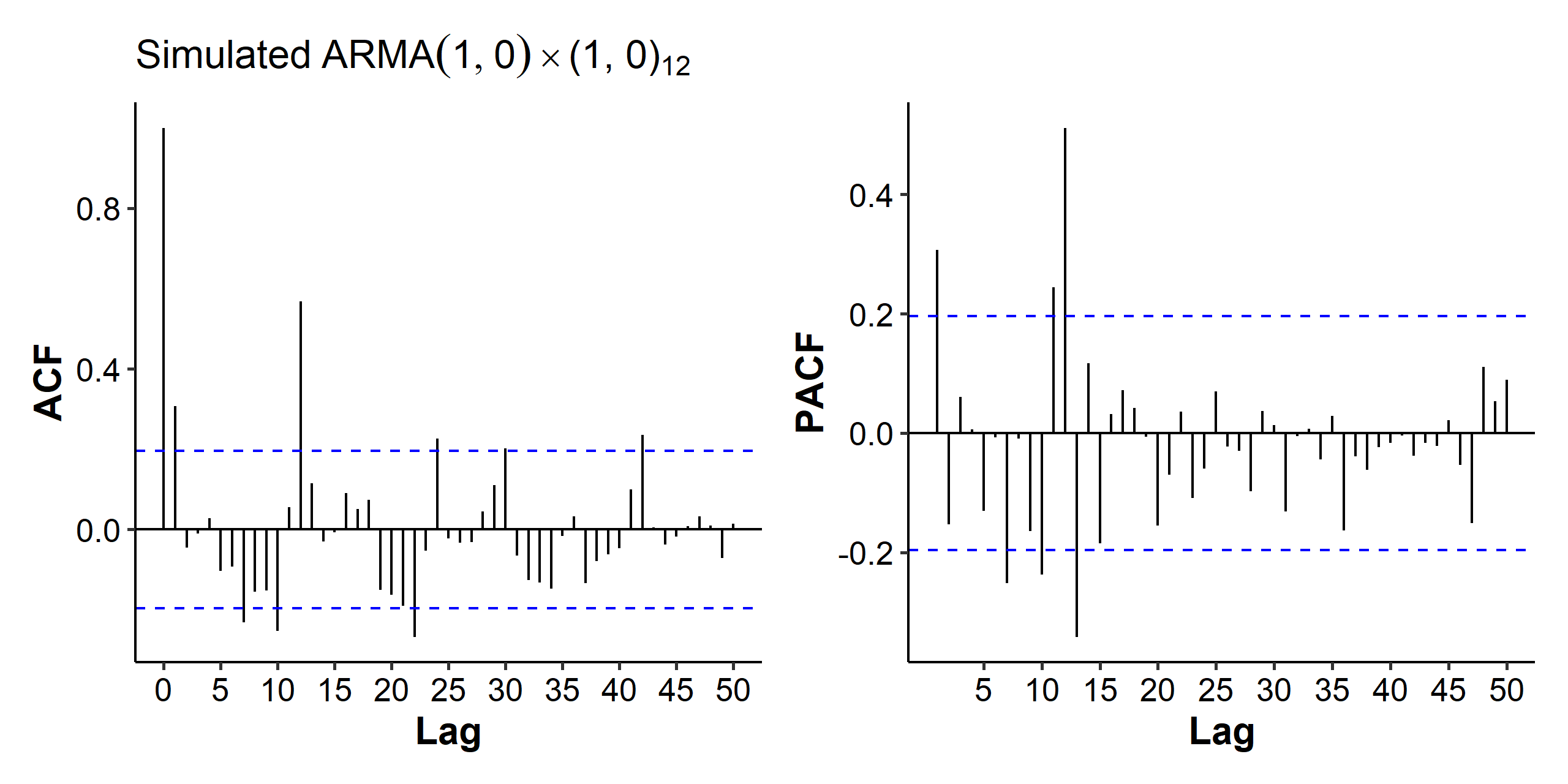
Simulated examples
So far we’ve been looking at plots of the theoretical ACF and PACF, and it’s already difficult in some cases to identify the orders. If we check the ACF of simulated data, it gets even messier:
| |
As we can see here, the tailing off at multiples of 12 in the ACF and the spike at lag 12 in the PACF coming from the seasonal AR(1) is still visible. Patterns from the regular AR(1) could also be seen, but clearly it’s much more challenging to identify them compared with the third example above.
If we look at the plots for 100 observations simulated from the following model:
$$ (1 - 0.7B)X_t = (1 + 0.8B^{12})(1 - 0.5B)Z_t $$
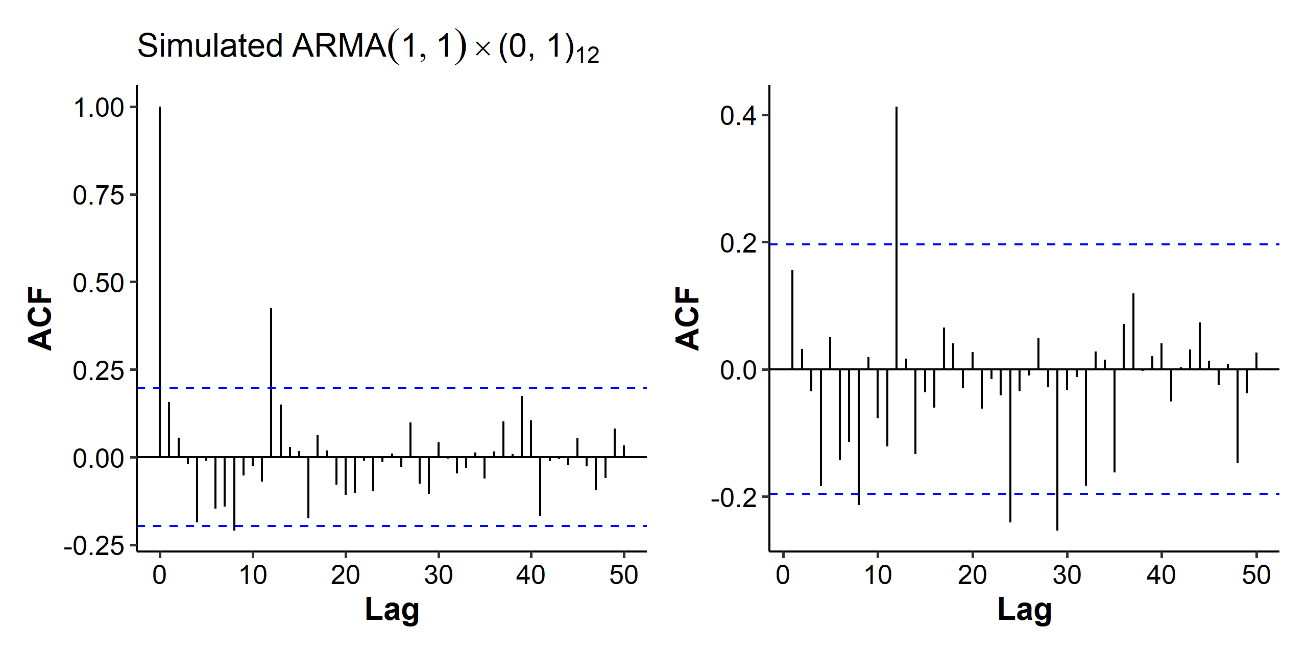
Once again the patterns are not so clear-cut. We can also fit the true model and see how close the estimated parameters are:
| |
Seasonal ARIMA
The idea behind the “I” in the seasonal ARIMA (SARIMA) model is the same as when we combined differencing and ARMA models. If we observe a seasonal pattern in the time series plot, and the ACF slowly decreasing at multiples of the period, then we might want to apply seasonal differencing.
Seasonal differencing
The seasonal difference is denoted $\nabla^S = 1 - B^S$. For example,
$$ (1 - B^{12})X_t = X_t - X_{t-12} $$
This difference above is used with monthly data that exhibits seasonality. The idea is that differences from the previous year may be (on average) about the same for each month of a year.
We have to decide the period $S$ in advance. For quarterly or monthly data, it’s straightforward to just use $S = 4$ or $S = 12$. For other more complicated cases, we’re going to use periodograms to help determine the period in a later chapter.
Formally speaking, suppose our model can be decomposed into a seasonal component and white noise
$$ X_t = S_t + Z_t, \quad t = 1, 2, \cdots, T $$
where $E(Z_t) = 0$, $S_{t+d} = S_t$, and $\sum_{j=1}^d S_j = 0$. Here $d$ is the period, so we’re assuming the seasonal effect in say May this year is the same as the effect in May of last year. Then, to eliminate the seasonal component by differencing, we may use the lag-$d$ differencing operator:
$$ (1 - B^d)X_t = X_t - X_{t-d} = Z_t - Z_{t-d} $$
If a trend and a seasonal component appear together, we may remove the seasonal trend with seasonal differencing3, and then remove the trend by applying a regression model, nonparametric smoothing, or regular differencing.
Seasonal data simulation
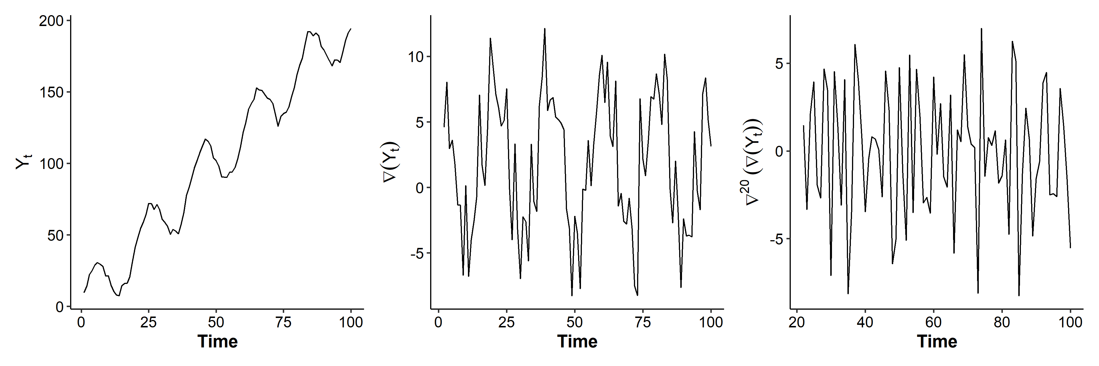
Let’s try simulating a series and applying seasonal differencing on it. Our data generating model is
$$ Y_t = 1 + 2t + 20\sin(0.1\pi t) + X_t, \quad X_t \sim MA(1) = Z_t + 0.5 Z_{t-1} $$
The 1 + 2t part is a linearly increasing trend, and the sin() part is a seasonal component. The period is $2\pi / 0.1\pi = 20$.
| |
The same function diff() is used for differencing and seasonal differencing.
| |
After regular differencing, the increasing trend is removed from $Y_t$, but there’s still a seasonal trend. The deseasonalized series shows none of the patterns observed in y or dy.
SARIMA model
If $d$ and $D$ are non-negative integers, then $\{X_t\}$ is a seasonal $ARIMA(p, d, q) \times (P, D, Q)_s$ process with period $s$ if the differenced series $Y_t = (1 - B)^d (1 - B^s)D X_t$ is an ARMA process. The full model is
$$ \phi(B)\Phi(B)(1 - B)^d(1 - B^s)^D X_t = \theta(B)\Theta(B)Z_t $$
where we have the terms in the order of regular AR, seasonal AR, regular differencing, seasonal differencing, regular MA and seasonal MA. Typically we set $D = 1$.
For example, the model $SARIMA(1, 0, 1) \times (0, 1, 1)_6$ can be written as
$$ (1 - \phi B) (1 - B^6)X_t = (1 + \theta B)(1 + \Theta B^6)Z_t, $$
and the model $SARIMA(0, 1, 2) \times (1, 1, 0)_{12}$ can be written as
$$ (1 - \Phi B^{12}) (1 - B)(1 - B^{12}) X_t = (1 + \theta_1 B + \theta_2 B^2)Z_t. $$
If we increase some of the orders to two $(0, 1, 2) \times (2, 2, 1)_{12}$, the model gets a lot more complicated:
$$ (1 - \Phi_1 B^{12} - \Phi_2 B^{24}) (1 - B) (1 - B^{12})^2 X_t = (1 + \theta_1 B + \theta_2 B^2)(1 + \Theta B^{12})Z_t $$
Multiplicative means that we’re constructing the regular and seasonal AR/MA polynomials separately and then multiplying them together. Consider the simplest case of $(0, 0, 1) \times (0, 0, 1)_{12}$, we have
$$ \begin{aligned} X_t &= (1 + \theta B)(1 + \Theta B^{12})Z_t \\ &= Z_t + \theta Z_{t-1} + \Theta Z_{t-12} + \theta\Theta Z_{t-13} \end{aligned} $$
In this multiplicative case, we only need to estimate two parameters: $\theta$ and $\Theta$. If this was additive, it would be an MA(13) model.
SARIMA in R
In R, we use the same arima() function for SARIMA models, only this time we need to specify one more parameter seasonal. Just like what we did at the end of this section, the parameter should be a named list with elements order and period where order is a numeric vector of length 3 specifying $P$, $D$, and $Q$.
When analyzing a series, the procedure is basically the same as that for the ARIMA model. One nuisance is the ADF test should be performed on the deseasonalized (but not regular-differenced) data. Once all the orders are figured out, use the original series in the arima() function.
Examples of seasonal differencing
In real data analysis, we usually first determine $d$, $s$ and $D$, then $P$ and $Q$ from the ACF and PACF with $s$ lags, and finally $p$ and $q$ from the regular ACF and PACF. Here we are going to give some examples of applying seasonal differencing for different processes.
Stochastic trend
We have a seasonal random walk plus a white noise
$$ X_t = S_t + Z_t, \quad S_t = S_{t-s} + \epsilon_t $$
where $Z_t$ and $\epsilon_t$ are independent WNs with variances $\sigma^2$ and $\sigma_\epsilon^2$, respectively. Let’s see what happens after seasonal differencing:
$$ \begin{aligned} \nabla^s X_t &= X_t - X_{t-s} \\ &= S_t + Z_t - (S_{t-s} + Z_{t-s}) \\ &= S_t - S_{t-s} + Z_t - Z_{t-s} \\ &= \epsilon_t + Z_t - Z_{t-s} \end{aligned} $$
which is an $MA(1)_s$, a stationary series that’s a linear combination of normal random variables. In fact, we can replace $Z_t$ with any stationary time series, and seasonal differencing would still be able to remove the seasonal random walk trend.
Random walk and seasonal random walk
The second example adds a random walk to the previous one:
$$ X_t = M_t + S_t + Z_t, \quad S_t = S_{t-s} + \epsilon_t, \quad M_t = M_{t-1} + \xi_t $$
where $Z_t$, $\epsilon_t$ and $\xi_t$ are independent WNs. To remove the trends, we need regular differencing and seasonal differencing:
$$ \begin{aligned} \nabla \nabla^s X_t &= \nabla(M_t + S_t + Z_t - M_{t-s} - S_{t-s} - Z_{t-s}) \\ &= \nabla(M_t - M_{t-s} + \epsilon_t + Z_t - Z_{t-s}) \\ &= (M_t - M_{t-s} + \epsilon_t + Z_t - Z_{t-s}) - (M_{t-1} - M_{t-s-1} + \epsilon_{t-1} + Z_{t-1} - Z_{t-s-1}) \\ &= \xi_t - \xi_{t-s} + \epsilon_t - \epsilon_{t-1} + Z_t - Z_{t-1} - Z_{t-s} + Z_{t-s-1} \end{aligned} $$
The remaining part is again statioary. In fact, it’s a SARIMA $(0, 0, 1) \times (0, 0, 1)_s$ process.
This is the opposite of the definition of frequency in physics, where this would be called the period and its inverse would be called the frequency. ↩︎
Here’s the R code for plotting the theoretical ACF and PACF.
↩︎1 2 3 4 5 6 7 8 9 10 11 12 13 14 15 16 17 18gg_acf_pacf <- function(x_acf, x_pacf, title) { p1 <- enframe(x_acf) %>% mutate_all(as.numeric) %>% ggplot(aes(x = name, y = value)) + geom_segment(aes(x = name, xend = name, y = 0, yend = value)) + geom_hline(yintercept = 0) + scale_x_continuous(breaks = seq(0, 50, 5)) + labs(x = "Lag", y = "Theoretical ACF") p2 <- enframe(x_pacf) %>% mutate_all(as.numeric) %>% ggplot(aes(x = name, y = value)) + geom_segment(aes(x = name, xend = name, y = 0, yend = value)) + geom_hline(yintercept = 0) + scale_x_continuous(breaks = seq(5, 50, 5)) + labs(x = "Lag", y = "Theoretical PACF") (p1 + ggtitle(title)) | p2 }It doesn’t really matter which differencing comes first. We can also remove the regular trend first and then deal with the seasonal trend. ↩︎
| Nov 17 | Spectral Analysis | 9 min read |
| Nov 02 | Decomposition and Smoothing Methods | 14 min read |
| Oct 09 | Variability of Nonstationary Time Series | 13 min read |
| Oct 05 | ARIMA Models | 9 min read |
| Sep 30 | Mean Trend | 13 min read |