Variability of Nonstationary Time Series

Oct 9, 2020

13 min read

Mar 11, 2022 15:59 UTC

Using the Box-Cox power transformation to stabilize the variance. At the end of this section, the standard procedure for fitting an ARIMA model is discussed.

In most of the chapter we’ve been talking about the mean trend of a time series and various methods of detecting and removing it. However, there’s another type of nonstationarity where the variability of a time series change with the mean level over time.

Recall that in linear regression we apply a log-transformation on $y$ when the variance of the residuals increases as $\hat{y}$ increases. Similar techniques can be applied for time series data. Here we’re talking about global changes – if the variance changes locally, then a transformation wouldn’t help and different methods would be needed to stabilize the variance.

Log transformation

We’ll use the AirPassengers dataset in R to show how the variability of a time series could be stabilized.

Monthly totals of international airline passenger numbers from 1949 to 1960.

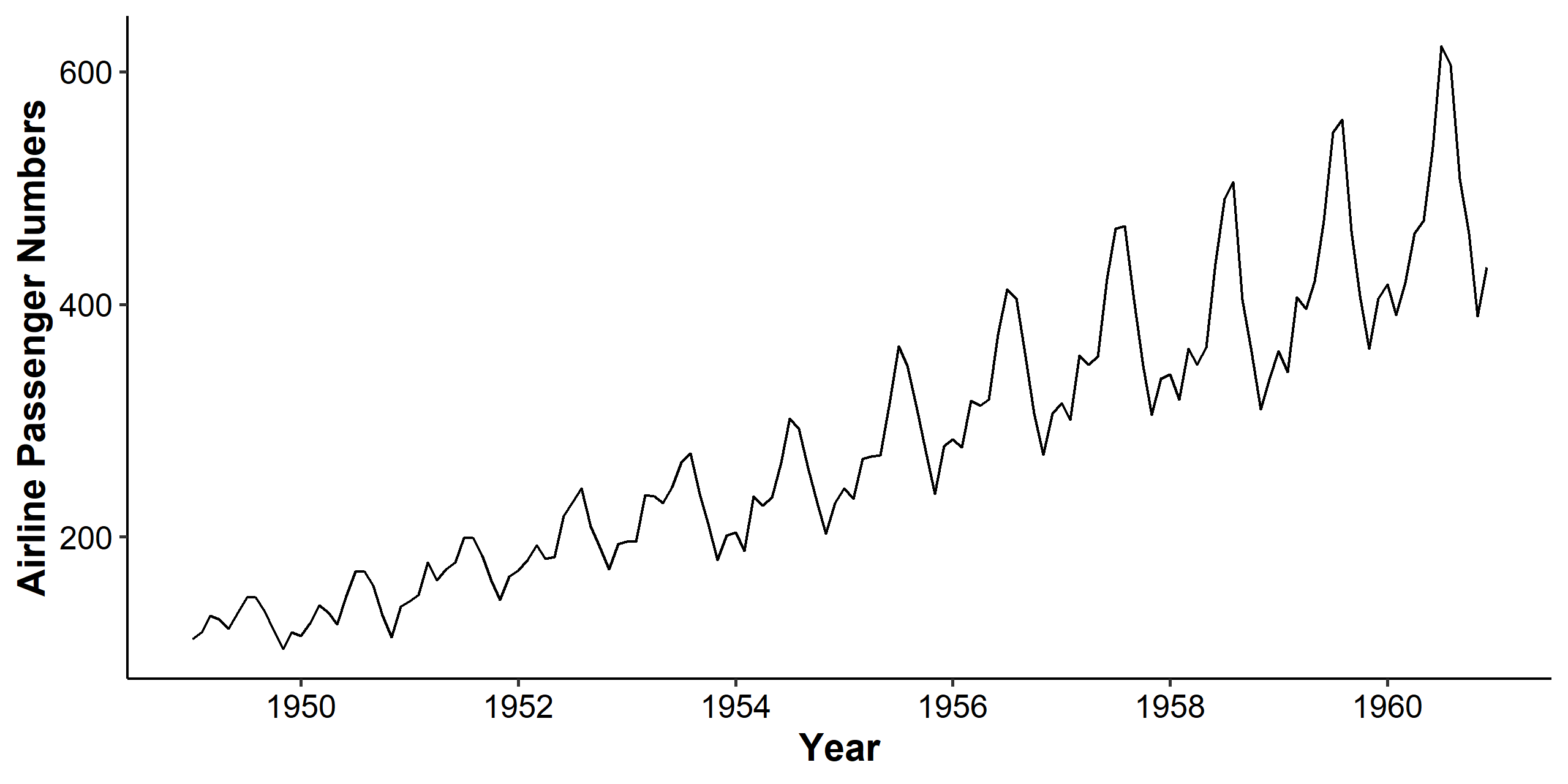
We can see clearly from the time series plot that the mean and variance both increase over time, and there’s a seasonal pattern involved. The increasing mean trend can be handled by differencing, and the seasonal pattern will be discussed in the next chapter.

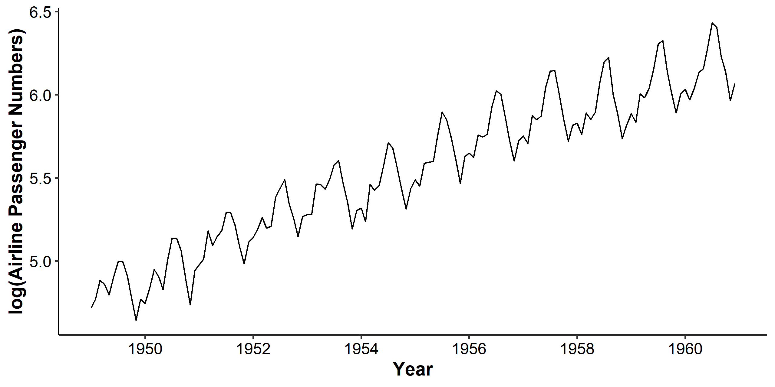
For stabilizing the variance, we can log-transform the dataset. As we can see below, the mean still increases, but the variance becomes stable across the years.

Log-transformed Monthly totals of international airline passenger numbers from 1949 to 1960.

Log-transformation works under the following assumption:

$$ E(X_t) = \mu_t, \quad Var(X_t) = \mu_t^2 \sigma^2 $$

To demonstrate this we are going to need a Taylor expansion of a smooth function $f(x)$ at $x_0$. We will only use the first order approximation of $f(x)$:

$$ f(x) = f(x_0) + f’(x_0)(x - x_0) + \frac{f’’(x_0)}{2!}(x - x_0)^2 + \cdots $$

Now we plug in $x_0 = \mu_t$.

$$ \begin{gathered} \log X_t \approx \log \mu_t + \frac{1}{\mu_t}(X_t - \mu_t) \\ E(\log X_t) \approx E(\log \mu_t) + \frac{1}{\mu_t}E(X_t - \mu_t) = \log \mu_t \\ Var(\log X_t) \approx \frac{1}{\mu_t^2}Var(X_t - \mu_t) = \frac{\mu_t^2\sigma^2}{\mu_t^2} = \sigma^2 \end{gathered} $$

So the variance becomes constant after taking the log-transform. We usually apply log-transformation when the variance of the series increases over time. After log-transformation, we can remove the remaining linear trend through differencing. We’ll discuss seasonal patterns in the next chapter.

Box-Cox power transformation

The log-transformation is a special case of a broader class called the Box-Cox power transformation. The Box-Cox transform is given by

$$ Y_t = \frac{X_t^\lambda - 1}{\lambda} $$

We apply different transformations when $\lambda$ takes different values:

$$ \begin{gathered} \lambda = -1 \Longrightarrow Y_t = \frac{1}{X_t} \\ \lambda = -0.5 \Longrightarrow Y_t = \frac{1}{\sqrt{X_t}} \\ \lambda = 0 \Longrightarrow Y_t = \log X_t \\ \lambda = 0.5 \Longrightarrow Y_t = \sqrt{X_t} \\ \lambda = 1 \Longrightarrow Y_t = X_t \end{gathered} $$

As indicated above, this method requires the time series $X_t$ to be positive. If there exists negative values, a certain constant can be added. In R, we can use FitAR::BoxCox() to find the MLE and a 95% confidence interval for $\lambda$.

Example of sunspot dataset

We’ll apply what we discussed to the sunspot dataset. The dataset contains 289 observations of yearly numbers of sunspots from 1700 to 1988 (rounded to one digit).

Time series plot

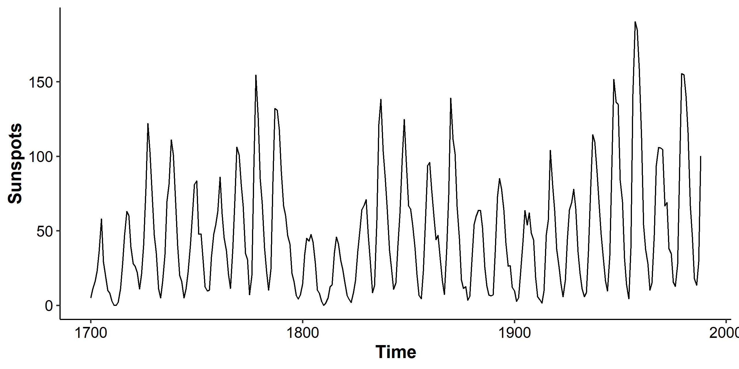
The mean looks somewhat stationary, but the variance is clearly changing over time, so we consider the Box-Cox transformation.

Transformation and differencing

1
2
3
4
5
library(FitAR)

data("sunspot.year")
BoxCox(sunspot.year)
#  minimum data value <= 0 so -min+0.25 added to all values

Relative likelihood function as well as the MLE and a 95% confidence interval for $\lambda$ in the Box-Cox power transformation.

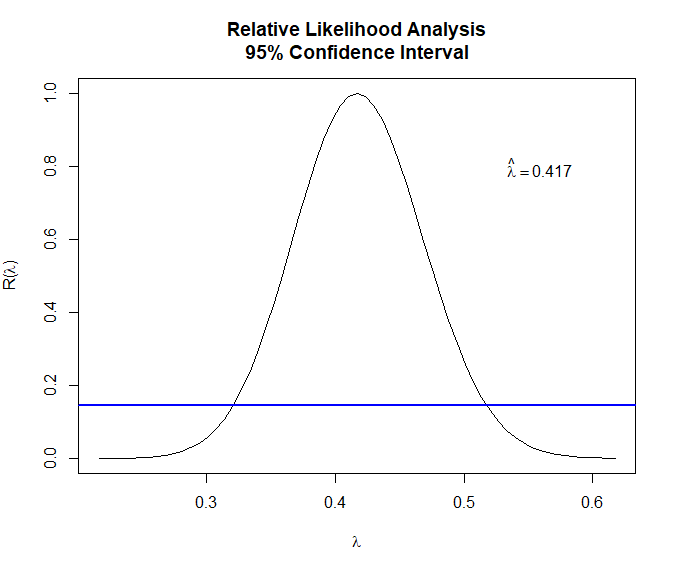
The MLE is $\hat\lambda = 0.417$ and the 95% CI covers 0.35-0.5. We may try $\lambda = 0.5$ and take the square root of the original series so it’s easier to interpret¹.

1
2
sp2 <- sqrt(sunspot.year)
plot_time_series(sp2)

Time series plot, ACF and PACF of the square-root transformed sunspot dataset.

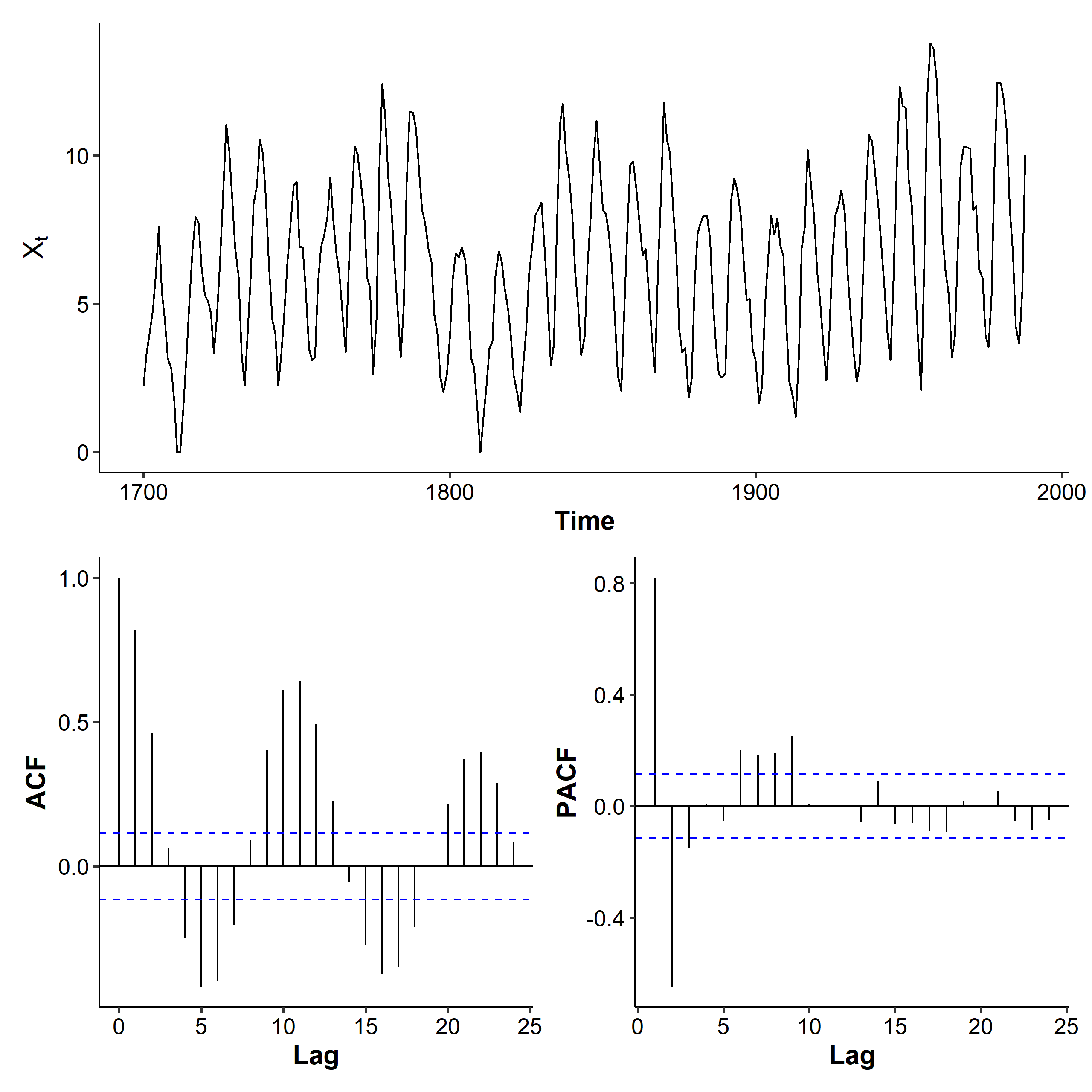
The variance of the transformed series is a lot stabler, although at some points (e.g. year 1800) it’s still not constant. The ACF decreases with a sine wave pattern, and the PACF has spikes at lags 1, 2, and up[ to lag 9. AR(9) is a candidate for this dataset.

We can use the ADF test to check if we need differencing. The p-value is smaller than 0.01, so we reject the null and treat the transformed series as stationary, thus no differencing is needed.

1
2
3
4
5
6
7
8
9
tseries::adf.test(sp2)
#     Augmented Dickey-Fuller Test

# data:  sp2
# Dickey-Fuller = -4.5857, Lag order = 6, p-value = 0.01
# alternative hypothesis: stationary

# Warning message:
# In tseries::adf.test(sp2) : p-value smaller than printed p-value

Train-test split and model fitting

We’re going to use the transformed data from now on. A 90-10 split is applied to prepare for calculating the MAPE later. The ar() function can be used to fit an AR model and check the coefficients. We set the order.max parameter as 10 because the last spike in the PACF was at lag 9.

 1
 2
 3
 4
 5
 6
 7
 8
 9
10
11
12
13
14
15
16
17
18
19
sp2_train <- sp2[1:260]
sp2_test <- sp2[261:289]

ar(sp2_train, order.max = 10)

# Call:
# ar(x = sp2_train, order.max = 10)

# Coefficients:
#       1        2        3        4        5        6        7        8        9
#  1.1737  -0.4003  -0.1475   0.1198  -0.1175   0.0667  -0.0080  -0.0441   0.1986

# Order selected 9  sigma^2 estimated as  1.378

ar(sp2_train, order.max = 10)$aic
#          0          1          2          3          4          5          6
# 456.131797 169.903951  24.512997  20.923631  22.822884  24.787340  20.929871
#          7          8          9         10
#  16.727759   8.460730   0.000000   1.686213

Among the 10 different AR orders, the ar() function selected order 9 as the best model based on its lowest AIC. Note that since some of the coefficients are very small, there’s room for improvement by setting some of those to zero in our model.

It’s obvious from the time series plot that the mean is not zero, but we can use a t-test to make sure:

 1
 2
 3
 4
 5
 6
 7
 8
 9
10
11
t.test(sp2_train)
# 	One Sample t-test

# data:  sp2_train
# t = 34.844, df = 259, p-value < 2.2e-16
# alternative hypothesis: true mean is not equal to 0
# 95 percent confidence interval:
#  5.852841 6.554005
# sample estimates:
# mean of x
#  6.203423

So we will include the intercept term. Now we can estimate the parameters in the AR(9) model:

 1
 2
 3
 4
 5
 6
 7
 8
 9
10
11
12
13
14
15
16
m1 <- arima(sp2_train, order = c(9, 0, 0), include.mean = T)
m1
# Call:
# arima(x = sp2_train, order = c(9, 0, 0), include.mean = T)

# Coefficients:
#          ar1      ar2      ar3     ar4      ar5      ar6     ar7      ar8     ar9
#       1.2290  -0.4823  -0.1405  0.2562  -0.2111  -0.0337  0.1753  -0.1548  0.2490
# s.e.  0.0601   0.0965   0.1004  0.1019   0.1023   0.1036  0.1044   0.1006  0.0631
#       intercept
#          6.2220
# s.e.     0.5391

# sigma^2 estimated as 1.08:  log likelihood = -380.99,  aic = 783.98

gg_diagnostic(m1)

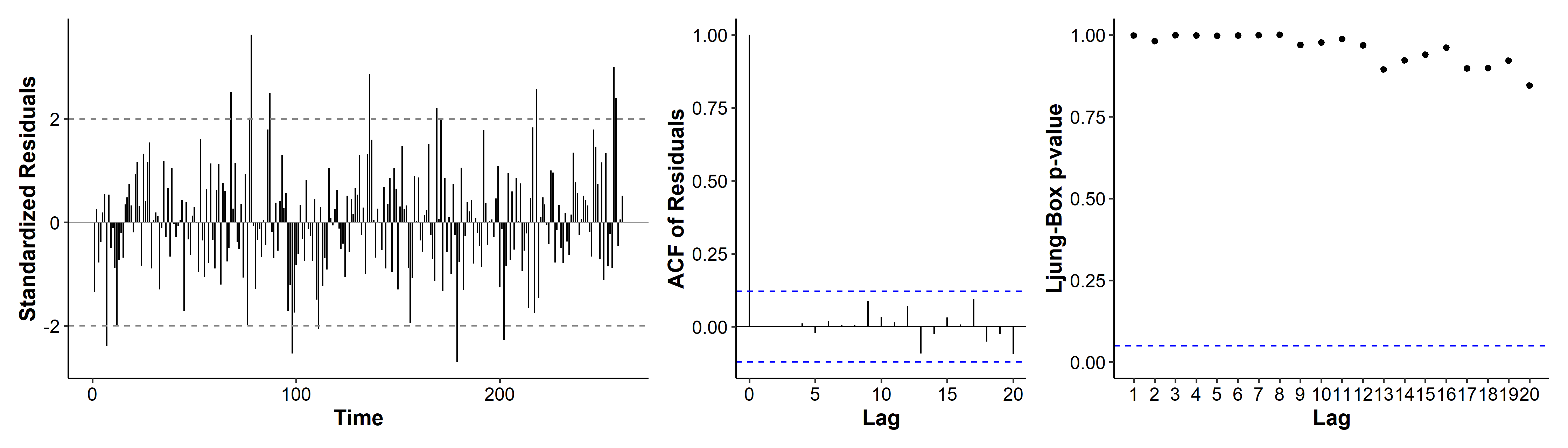
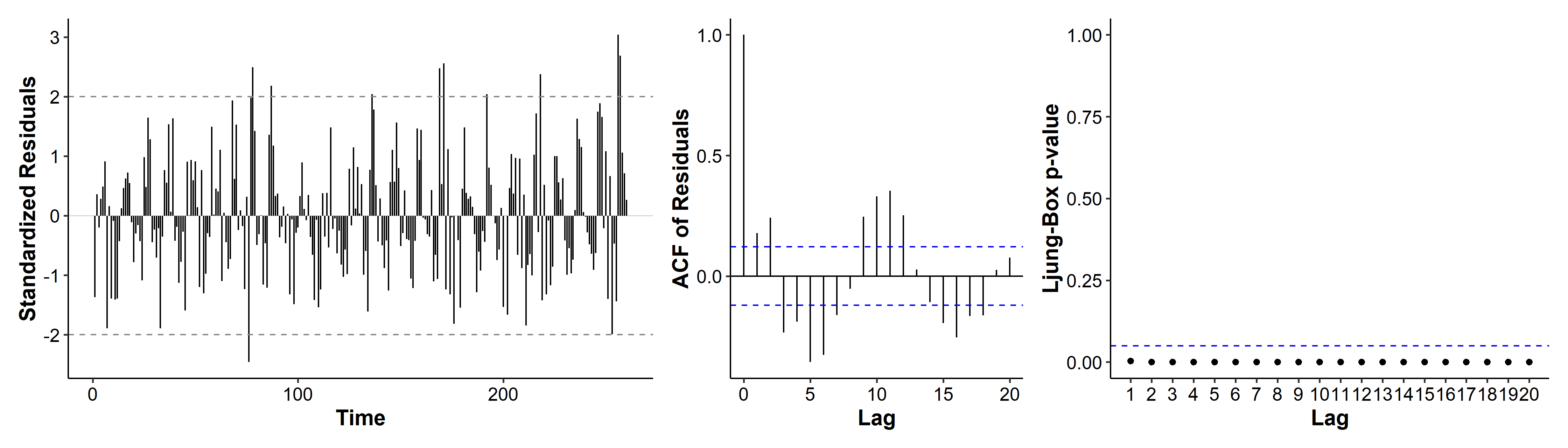
In the diagnostic plots, quite a few standardized residuals are over the $\pm 2$ range. the ACF only has a spike at lag 0, indicating no autocorrelation in the residuals. All p-values for the Ljung-Box tests are very high. Overall there doesn’t seem to be major violations of our model assumptions.

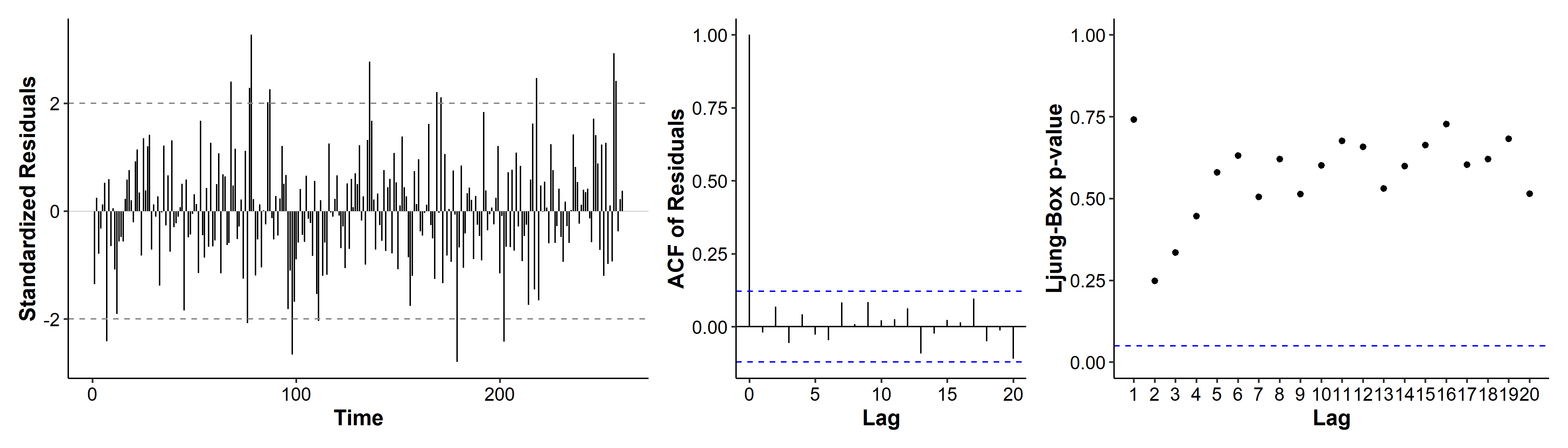
As we said earlier, we can try to reduce the number of parameters in our model. By looking and the coefficients and their standard errors, we may eliminate some parameters. For example, the ar3 coefficient’s CI includes zero, so we may drop it from our model. The same goes for ar6, ar7 and ar8.

 1
 2
 3
 4
 5
 6
 7
 8
 9
10
11
12
13
m2 <- arima(sp2_train, order = c(9, 0, 0), include.mean = T,
            fixed = c(NA, NA, 0, NA, NA, 0, 0, 0, NA, NA))
m2
# Call:
# arima(x = sp2_train, order = c(9, 0, 0), include.mean = T, fixed = c(NA, NA,
#     0, NA, NA, 0, 0, 0, NA, NA))

# Coefficients:
#          ar1      ar2  ar3     ar4      ar5  ar6  ar7  ar8     ar9  intercept
#       1.2360  -0.5542    0  0.1110  -0.1173    0    0    0  0.2048     6.2195
# s.e.  0.0572   0.0690    0  0.0702   0.0564    0    0    0  0.0285     0.5154

# sigma^2 estimated as 1.103:  log likelihood = -383.68,  aic = 781.36

We’ve gone from 10 coefficients (9 + intercept) to 6. The diagnosis plots are not too different, and the model assumptions are still met.

A third model we may consider is ARMA(1, 1), if we consider the patterns in Figure 5 to be tail-off.

 1
 2
 3
 4
 5
 6
 7
 8
 9
10
11
m3 <- arima(sp2_train, order = c(1, 0, 1), include.mean = T)
m3
# Call:
# arima(x = sp2_train, order = c(1, 0, 1), include.mean = T)

# Coefficients:
#          ar1     ma1  intercept
#       0.7503  0.5282     6.2216
# s.e.  0.0438  0.0438     0.4999

# sigma^2 estimated as 1.78:  log likelihood = -444.76,  aic = 897.52

The AIC is a lot higher than before! if we look at the diagnostic plots, the ACF has multiple spikes, and the p-values are all below 0.05. ARMA(1, 1) is thus not a good candidate model.

Diagnostic plots for the ARMA(1, 1) model.

Model selection

To further compare the other two models, we can check their AIC, BIC, number of parameters, and MAPE. The reduced model performs better in terms of all four criteria.

Criteria	AR(9)	Reduced
AIC	783.9829	781.3608
BIC	823.1504	806.2856
# parameters	10	6
MAPE	0.1671	0.1657

We then fit the entire dataset and get our final model:

$$ (1 - 1.2278B +0.5479B^2 - 0.1132B^4 +0.1149B^5 - 0.2154B^9)(\sqrt{X_t} - 6.3985) = Z_t $$

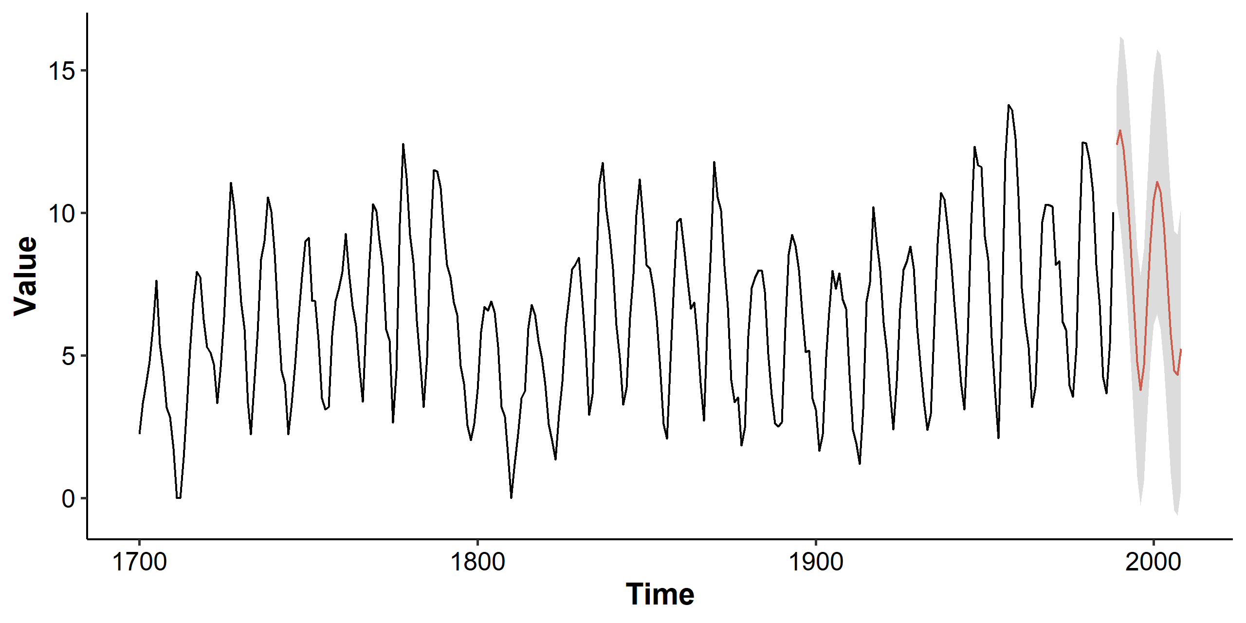
with $\hat\sigma^2 = 1.116$. We can use this final model to predict future values. Note that the y-axis is still transformed, and we can take the square to visualize the original scale. We can also simplify the plotting code using the plot(forecast(model, 20)) function from the R package forecast. The function also takes a lambda parameter that could automatically transform the series back to its original scale.

20 forecasts for the sunspots dataset. The y-axis is square-root transformed.

Summary

The general procedure for model fitting is as follows.

Time series plot. We want to first check for mean and variance changes, as well as seasonal or other patterns.
Transformation. Using Box-Cox we can determine if transformation is necessary for our data. If it is then we use the transformed data from this step onwards.
Divide the data. Apply a train-test split on the (transformed) data so that we can calculate the MAPE (or other metrics) for our models. The following steps should only use the training set.
Check whether differencing is needed. Using the ts plot, ACF and the ADF test to determine if we need to difference the data.
Determine $p$ and $q$ for the ARIMA model. Use patterns in the ACF and PACF to find candidate models.
Fit models. In model fitting we should use un-differenced data, because ARIMA will take care of the differencing.
Model diagnosis. A candidate model shouldn’t have any of its assumptions violated.
Model selection. Use the AIC, BIC, parameter number and MAPE to find the best model. The testing set will be used in this step.
Build final model. Use the entire dataset to update the selected model.
Use model for forecasting. Don’t forget to include prediction intervals.

The helper functions for plotting and the session info are given below.

  1
  2
  3
  4
  5
  6
  7
  8
  9
 10
 11
 12
 13
 14
 15
 16
 17
 18
 19
 20
 21
 22
 23
 24
 25
 26
 27
 28
 29
 30
 31
 32
 33
 34
 35
 36
 37
 38
 39
 40
 41
 42
 43
 44
 45
 46
 47
 48
 49
 50
 51
 52
 53
 54
 55
 56
 57
 58
 59
 60
 61
 62
 63
 64
 65
 66
 67
 68
 69
 70
 71
 72
 73
 74
 75
 76
 77
 78
 79
 80
 81
 82
 83
 84
 85
 86
 87
 88
 89
 90
 91
 92
 93
 94
 95
 96
 97
 98
 99
100
101
102
103
104
105
106
107
108
109
110
111
112
113
114
115
116
117
118
119
120
121
122
123
124
125
126
127
128
129
130
131
132
133
134
135
136
137
138
139
140
141
142
143
144
145
146
147
148
149
150
151
152
153
154
155
library(FitAR)
library(tidyverse)
library(patchwork)

theme_set(
  ggpubr::theme_pubr() +
    theme(
      axis.title = element_text(face = "bold", size = 14)
    )
)

gg_acf <- function(object, acf.type = "ACF") {
  ci <- qnorm((1 + 0.95) / 2) / sqrt(object$n.used)  # 95% CI

  data.frame(
    Lag = as.numeric(object$lag),
    ACF = as.numeric(object$acf)
  ) %>%
    ggplot(aes(x = Lag, y = ACF)) +
    geom_segment(aes(x = Lag, xend = Lag, y = 0, yend = ACF)) +
    geom_hline(yintercept = 0) +
    geom_hline(yintercept = c(-ci, ci), linetype = "dashed", color = "blue") +
    ylab(acf.type)
}

gg_time_series <- function(x, lag.max = NULL, ylab = expression(X[t]), ACF = T) {
  x_acf <- acf(x, lag.max = lag.max, plot = F)
  x_pacf <- pacf(x, lag.max = lag.max, plot = F)

  p1 <- tibble(Timepoint = time(x), x = x) %>%
    ggplot(aes(Timepoint, x)) +
    geom_line() +
    xlab("Time") +
    ylab(ylab)

  if (ACF) {
    p2 <- gg_acf(x_acf, "ACF")
    p3 <- gg_acf(x_pacf, "PACF")
    p <- (p1 / (p2 | p3))
  } else {
    p <- p1
  }
  p
}

gg_diagnostic <- function (x.fit, gof.lag = 20, fit.df = 1) {
  # Get standardized residuals of the fit
  rs <- residuals(x.fit)
  stdres <- rs / sqrt(x.fit$sigma2)

  # Residual plot
  p1 <- stdres %>%
    enframe() %>%
    select(Time = name, Value = value) %>%
    ggplot(aes(x = Time, y = Value)) +
    geom_segment(aes(x = Time, xend = Time, y = 0, yend = Value)) +
    ylab("Standardized Residuals") +
    geom_hline(yintercept = 0, size = 0.2, color = "#888888") +
    geom_hline(yintercept = 2, linetype = "dashed", color = "#888888") +
    geom_hline(yintercept = -2, linetype = "dashed", color = "#888888")

  # ACF of the residuals
  x_acf <- acf(rs, lag.max = gof.lag, plot = F, na.action = na.pass)
  p2 <- gg_acf(x_acf, "ACF of Residuals")

  # p-values for the Ljung-Box statistic; default tsdiag() does it wrong.
  # Only fallback to default when lag <= # of parameters.
  lb <- data.frame(
    Lag = seq(gof.lag)
  ) %>%
    mutate(
      pval = map_dbl(Lag, function(x)
        Box.test(rs, lag = x, type = "Ljung-Box",
                 fitdf = ifelse(x <= fit.df, 0, fit.df))$p.value
      ))

  p3 <- ggplot(lb, aes(x = Lag, y = pval)) +
    geom_point() +
    geom_hline(yintercept = 0.05, linetype = "dashed", color = "blue") +
    scale_x_continuous(breaks = seq(gof.lag)) +
    scale_y_continuous(limits = c(0, 1)) +
    ylab("Ljung-Box p-value")

  (p1 | p2 | p3) + plot_layout(widths = c(2, 1, 1.5))
}

model_selection <- function(model, df_test) {
  pred <- predict(model, length(df_test))$pred
  res <- matrix(c(
    model$aic,
    BIC(model),
    mean(abs((df_test - pred) / df_test))
  ), nrow = 1)
  colnames(res) <- c("AIC", "BIC", "MAPE")
}

gg_forecast <- function(x, model, n.ahead = 5) {
  x.pred <- predict(model, n.ahead)
  x.pred.upper <- x.pred$pred + 1.96 * x.pred$se
  x.pred.lower <- x.pred$pred - 1.96 * x.pred$se

  dat.x <- data.frame(
    Time = time(x),
    Value = as.numeric(x)
  )

  dat.x.fore <- data.frame(
    Time = seq(max(time(x)) + 1, length.out = n.ahead),
    Value = as.numeric(x.pred$pred),
    Upper = x.pred.upper,
    Lower = x.pred.lower
  )

  ggplot(dat.x, aes(x = Time, y = Value)) +
    geom_line() +
    geom_line(data = dat.x.fore, color = "#E64B35") +
    geom_ribbon(data = dat.x.fore, aes(ymin = Lower, ymax = Upper),
                fill = "#888888", alpha = 0.3) +
    theme(legend.position = "none")
}

sessionInfo()
# R version 4.0.3 (2020-10-10)
# Platform: x86_64-w64-mingw32/x64 (64-bit)
# Running under: Windows 10 x64 (build 19041)

# Matrix products: default

# attached base packages:
# [1] stats     graphics  grDevices utils     datasets  methods   base

# other attached packages:
#  [1] patchwork_1.0.1 forcats_0.5.0   stringr_1.4.0   dplyr_1.0.2     purrr_0.3.4
#  [6] readr_1.4.0     tidyr_1.1.2     tibble_3.0.4    ggplot2_3.3.2   tidyverse_1.3.0
# [11] FitAR_1.94      bestglm_0.37.3  ltsa_1.4.6      leaps_3.1       lattice_0.20-41

# loaded via a namespace (and not attached):
#  [1] tseries_0.10-47   httr_1.4.2        jsonlite_1.7.1    splines_4.0.3
#  [5] foreach_1.5.0     carData_3.0-4     modelr_0.1.8      assertthat_0.2.1
#  [9] TTR_0.24.2        blob_1.2.1        cellranger_1.1.0  pillar_1.4.6
# [13] backports_1.1.10  glue_1.4.2        quadprog_1.5-8    ggsignif_0.6.0
# [17] rvest_0.3.6       colorspace_1.4-1  Matrix_1.2-18     pkgconfig_2.0.3
# [21] broom_0.7.1       haven_2.3.1       scales_1.1.1      openxlsx_4.2.2
# [25] grpreg_3.3.0      rio_0.5.16        generics_0.0.2    car_3.0-10
# [29] ellipsis_0.3.1    ggpubr_0.4.0      withr_2.3.0       cli_2.1.0
# [33] quantmod_0.4.17   survival_3.2-7    magrittr_1.5      crayon_1.3.4
# [37] readxl_1.3.1      fs_1.5.0          fansi_0.4.1       rstatix_0.6.0
# [41] xts_0.12.1        xml2_1.3.2        foreign_0.8-80    tools_4.0.3
# [45] data.table_1.13.0 hms_0.5.3         lifecycle_0.2.0   munsell_0.5.0
# [49] reprex_0.3.0      glmnet_4.0-2      zip_2.1.1         pls_2.7-3
# [53] compiler_4.0.3    rlang_0.4.8       grid_4.0.3        iterators_1.0.12
# [57] rstudioapi_0.11   gtable_0.3.0      codetools_0.2-16  abind_1.4-5
# [61] DBI_1.1.0         curl_4.3          R6_2.4.1          zoo_1.8-8
# [65] lubridate_1.7.9   shape_1.4.5       stringi_1.5.3     Rcpp_1.0.5
# [69] vctrs_0.3.4       dbplyr_1.4.4      tidyselect_1.1.0

We can also just use the MLE, e.g. bxcx(sunspot.year, lambda = 0.417). ↩︎

Nov 17	Spectral Analysis	9 min read
Nov 02	Decomposition and Smoothing Methods	14 min read
Oct 13	Seasonal Time Series	17 min read
Oct 05	ARIMA Models	9 min read
Sep 30	Mean Trend	13 min read