ARIMA Models

Previously we introduced ARMA models that combined the power of autoregressive series and moving average models. Recall that when modeling a series using the arima function, the order parameter had three integer components $(p, d, q)$ and we always set $d=0$. The three integers are the AR order, the degree of differencing, and the MA order.

Definition

The Autoregressive Integrated Moving Average (ARIMA) model uses an ARMA model after the $d^{th}$ order differencing. $X_t: ARIMA(p, d, q)$ can be expressed as $(1-B)^d X_t: ARMA(p, q)$, or

$$ \Phi(B)(1-B)^d X_t = \Theta(B)Z_t, $$

where

$$ \begin{gathered} \Phi(B) = 1 - \phi_1 B - \phi_2 B^2 - \cdots - \phi_p B^p \\ \Theta(B) = 1 + \theta_1 B + \theta_2 B^2 + \cdots + \theta_q B^q \end{gathered} $$

For example, an ARIMA(2, 1, 0) model is given by

$$ (1 - \phi_1 B - \phi_2 B^2)(1-B)X_t = Z_t $$

An ARIMA(1, 1, 2) model is given by

$$ (1 - \phi B)(1-B) X_t = (1 + \theta_1 B + \theta_2 B^2)Z_t $$

And an ARIMA(0, 2, 1) model:

$$ (1-B)^2 X_t = (1 + \theta B)Z_t $$

Finding the order

We’ll explain how to find the order of ARIMA models through some exercises. After this section we should be able to identify $p$, $d$ and $q$ when looking at a written model.

Unlike the ARMA model, it’s not easy to recognize the three orders together. To find the order of an ARIMA model, we need to convert the models to the canonical format and first determine $d$.

1. $X_t = X_{t-1} + Z_t + 0.2 Z_{t-1} - 0.5 Z_{t-2}$.

   $$ \begin{gathered} X_t - X_{t-1} = Z_t + 0.2 Z_{t-1} - 0.5 Z_{t-2} \\ (1-B)X_t = (1 + 0.2 B - 0.5B^2)Z_t \end{gathered} $$

   This is an ARIMA(0, 1, 2) model. The $(1-B)$ part should be considered as differencing and not AR(1).

2. $X_t = 1.7 X_{t-1} - 0.7 X_{t-2} + Z_t + 0.4 Z_{t-1}$.

   $$ \begin{gathered} X_t - 1.7 X_{t-1} + 0.7 X_{t-2} = Z_t + 0.4 Z_{t-1} \\ (1 - 1.7 B + 0.7 B^2)X_t = (1 + 0.4 B)Z_t \end{gathered} $$

   We can easily see the MA(1) order from the RHS. For the LHS, note that it contains a differencing term:

   $$ (1-0.7B)(1-B)X_t = (1 + 0.4B)Z_t $$

   So it’s not an ARMA(2, 1) model, but actually an ARIMA(1, 1, 1) model. Generally we check if $B=1$ is a root for the polynomial on the LHS.

3. $X_t = 1.6 X_{t-1} - 0.5 X_{t-2} - 0.1 X_{t-3} + Z_t$.

$$ (1 - 1.6B + 0.5 B^2 + 0.1 B^3)X_t = Z_t $$

There’s no MA part. $B=1$ is a solution for the LHS, so

$$ (1 - 0.6B - 0.1 B^2)(1-B)X_t = Z_t $$

$B=1$ is no longer a solution for $(1 - 0.6B - 0.1 B^2)$, so our model is ARIMA(2, 1, 0).

Simulated ARIMA series

In this section we’re going to simulate some ARIMA series with different parameters, and see if we can determine $d$ and then $p$ and $q$ from the ACF and PACF.

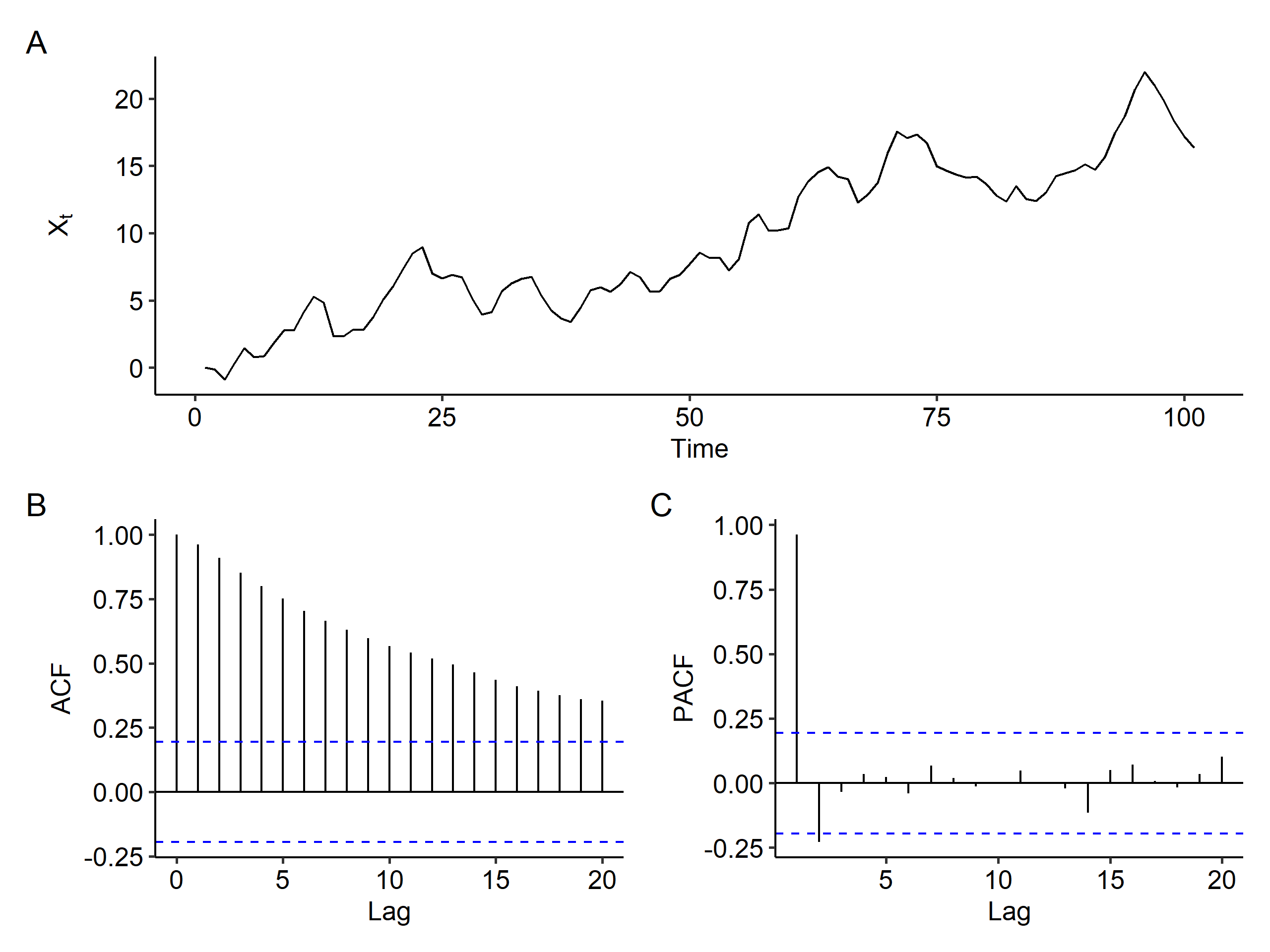
IMA(1, 1)

This is the same as an ARIMA(0, 1, 1) model and there’s no AR part. Our model is

$$ (1-B)X_t = (1 - 0.5B)Z_t $$

1
2
3
4

set.seed(1)
x <- arima.sim(list(order = c(0, 1, 1), ma = 0.5), n = 100)

plot_time_series(x)

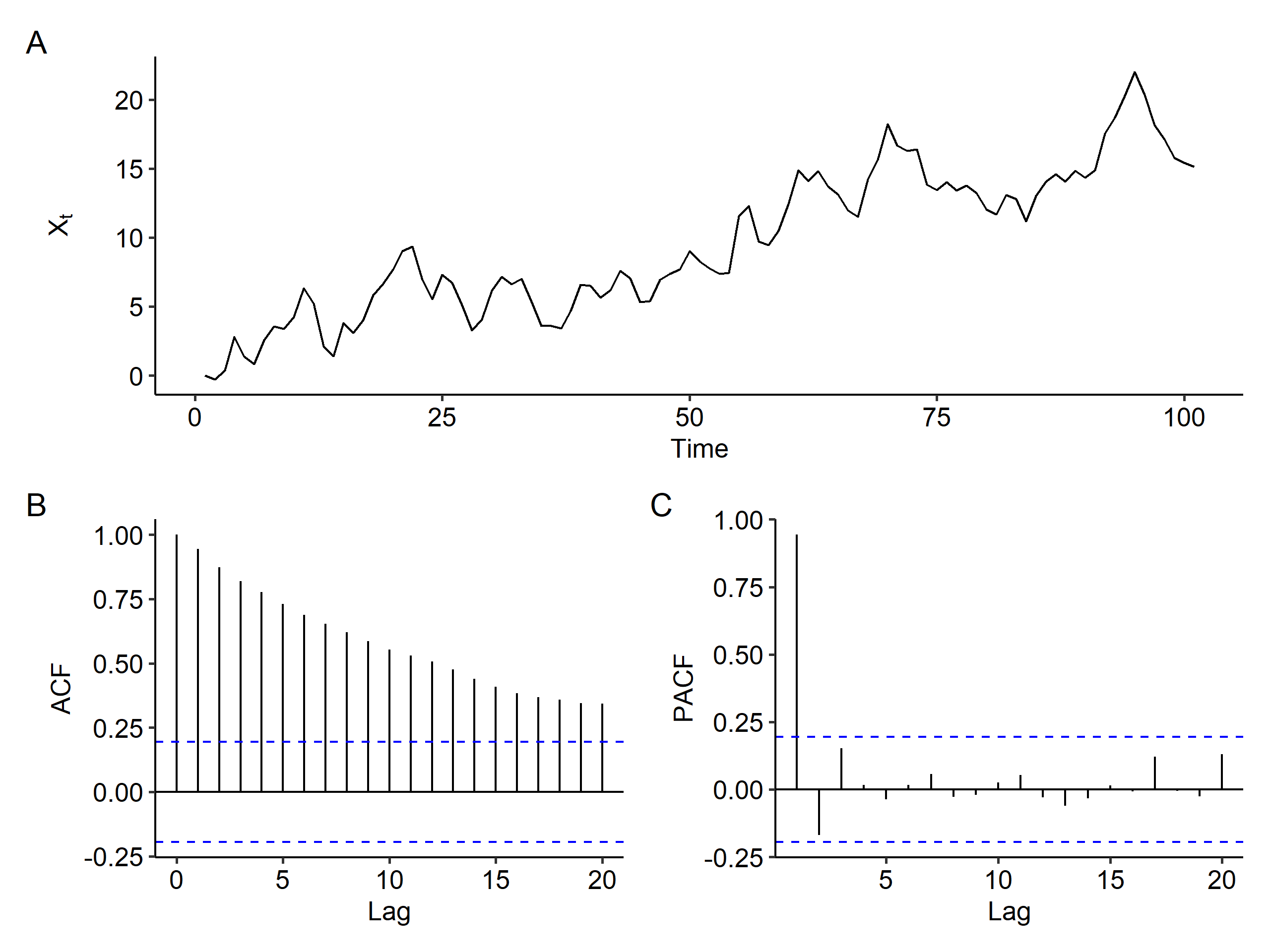
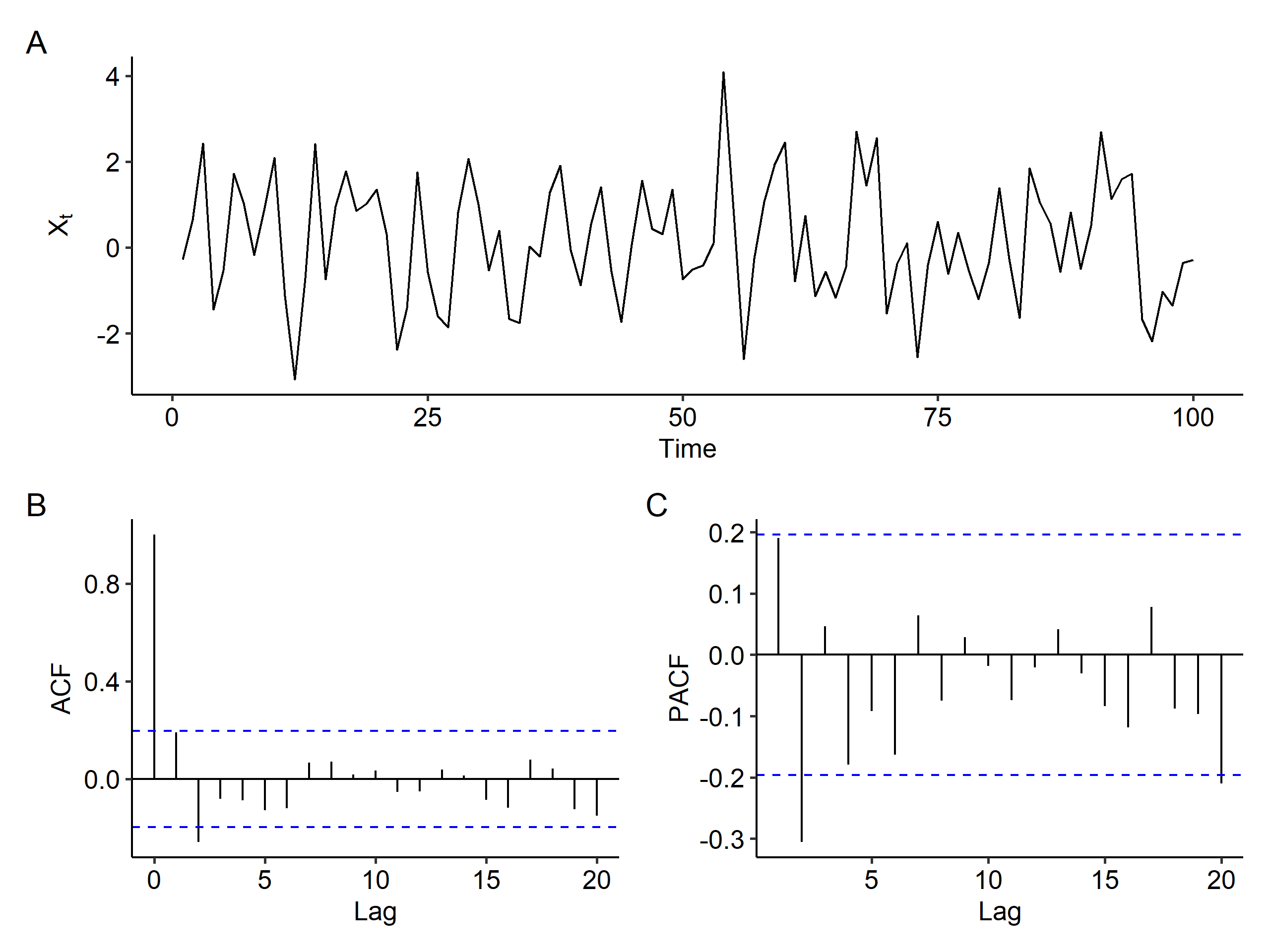
Plotting the time series, ACF and PACF¹, we can see that there’s a clear increasing trend and the ACF slowly decreases, both indicating that differencing is needed. There are three possibilities for the slowly decreasing ACF:

1. a mean trend needs to be removed,
2. random walk, and
3. a stationary process with very strong autocorrelation – long-range dependence (LRD) time series². In this case the PACF is also going to slowly decrease.

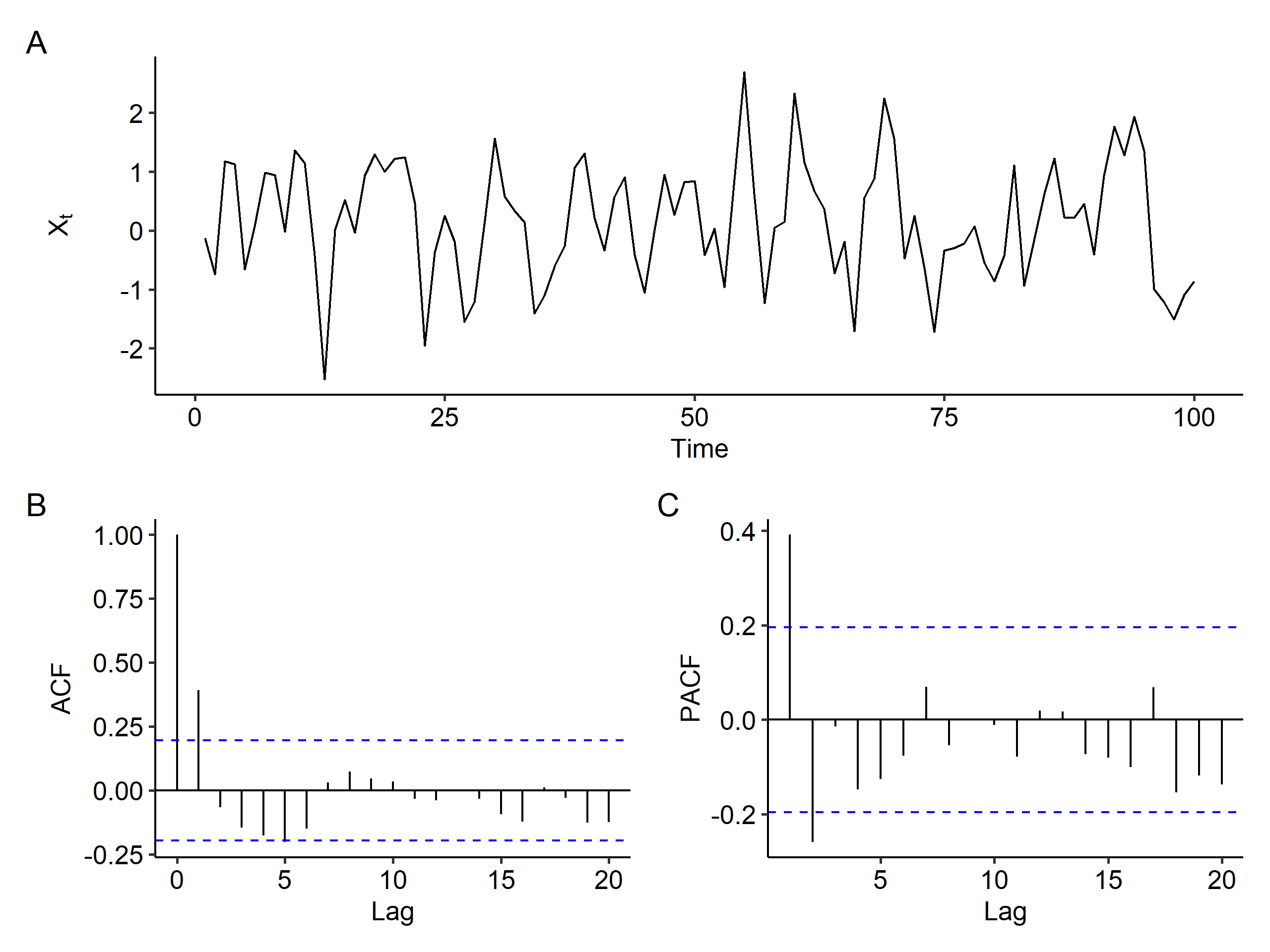
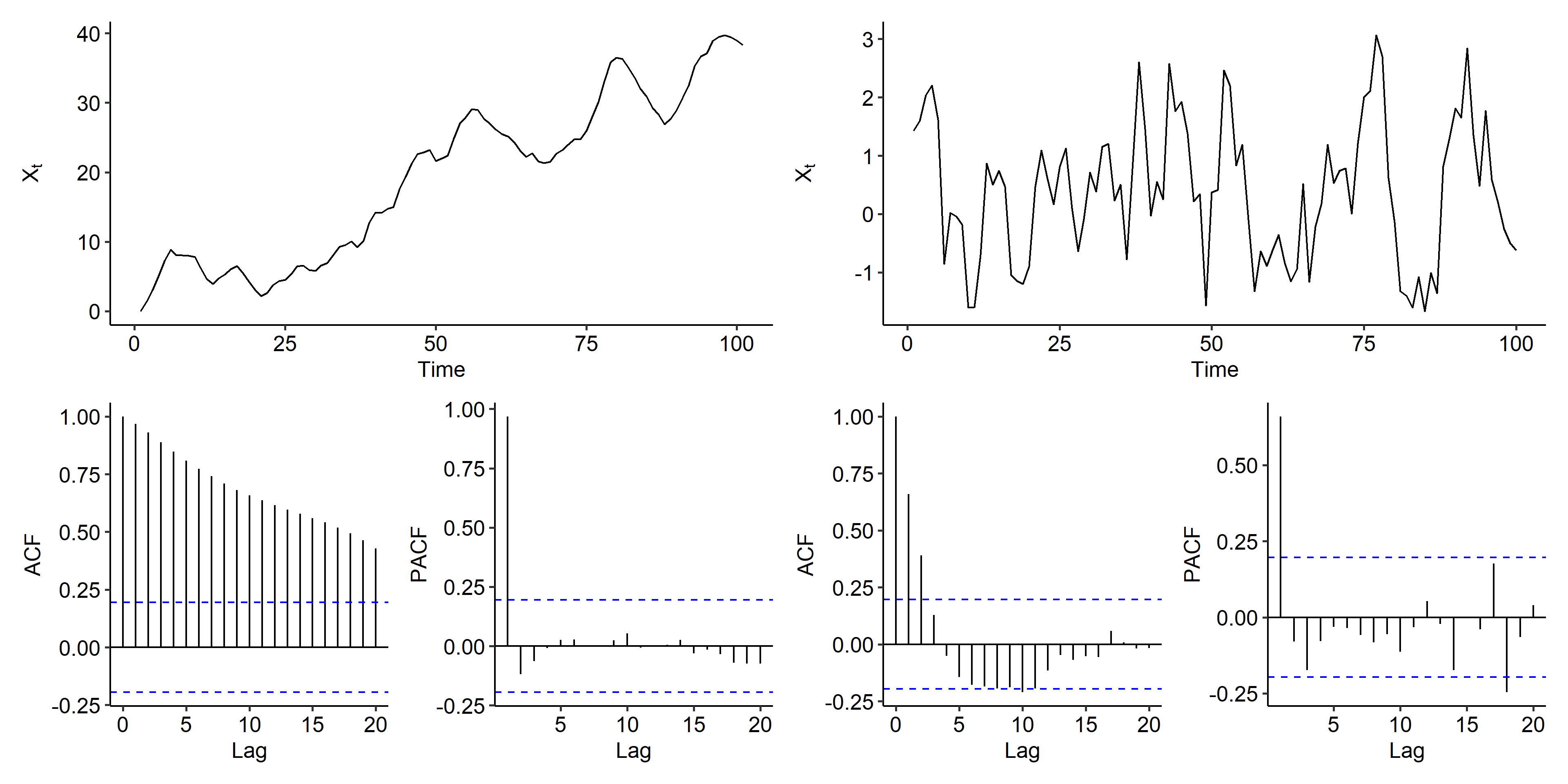
Now if we apply first order differencing, the increasing trend goes away. We see a spike at lag 1 in the ACF plot, and the PACF shows a tail-off pattern, so MA(1) is a good model³. A good candidate for the original series is ARIMA(0, 1, 1), which is our data generating process.

1
2

dx <- diff(x, differences = 1)
plot_time_series(dx)

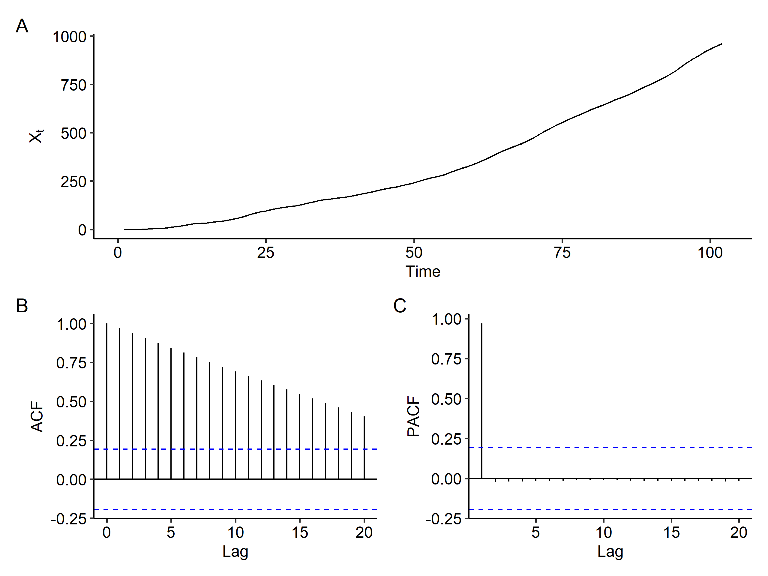
IMA(2, 2)

Our ARIMA(0, 2, 2) model is

$$ (1-B)^2 X_t = (1 + B - 0.6B^2)Z_t $$

1
2
3
4

set.seed(1)
x <- arima.sim(list(order = c(0, 2, 2), ma = c(1, -0.6)), n = 100)

plot_time_series(x)

Once again, there’s a clear increasing trend and the ACF slowly decreases. We definitely need differencing, but it’s hard to say the order of the differencing.

1
2

dx <- diff(x, differences = 1)
plot_time_series(dx)

After first order differencing, there’s still a trend in the time series plot, and the ACF still slowly decreases, although faster than before differencing. This suggests that maybe first order differencing was sufficient to remove the mean trend.

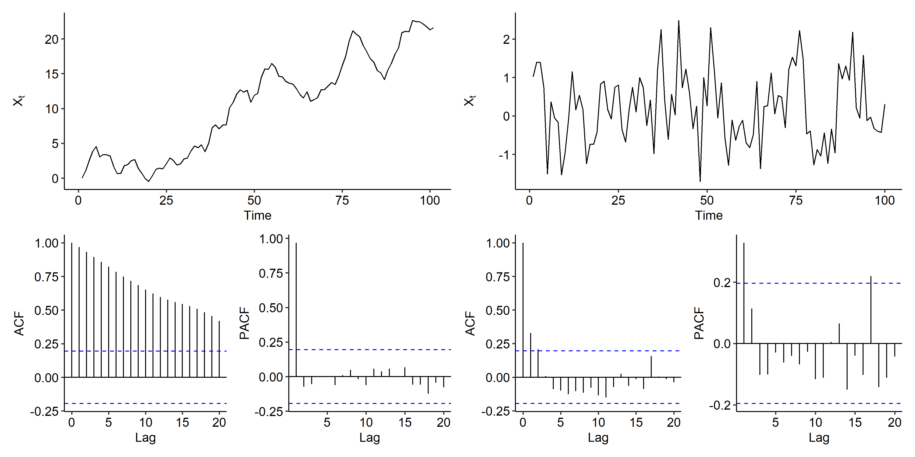
After second order differencing, however, we end up with a stationary process and the slowly decreasing pattern in the ACF is gone.

1
2

dx <- diff(x, differences = 2)
plot_time_series(dx)

So what’s the order of the model? After second order differencing, we can observe a spike at lag 2 in the ACF plot, and so does the PACF plot. It’s much harder to determine the order compared to the previous case, but an ARIMA(0, 2, 2) model might be suitable.

ARI(1, 1)

This time our model is

$$ (1 - 0.7B)(1-B)X_t = Z_t $$

Following the same process as above, we observe similar patterns in the original series, and the increasing trend is removed after the first order differencing. The ACF of the differenced series tails off, and the PACF is cut off after lag 1, suggesting an AR(1) model.

ARIMA(1, 1, 1)

Our final example is the following:

$$ (1 - 0.7B)(1-B)X_t = (1 - 0.4B)Z_t $$

The mean is stabilized after first order differencing, and both and ACF and PACF can be viewed as tail off patterns. Both ARIMA(1, 1, 1) and ARIMA(1, 1, 0) could be considered.

Estimation, diagnosis and forecasting

The procedure is exactly the same as before, except that we include a step of differencing now.

Estimation and diagnosis

Using the ARIMA(1, 1, 1) series as an example:

 1
 2
 3
 4
 5
 6
 7
 8
 9
10
11
12

set.seed(1)
x <- arima.sim(list(order = c(1, 1, 1), ar = 0.7, ma = -0.4), n = 100, sd = 3)
x.fit <- arima(x, order = c(1, 1, 1))
# Call:
# arima(x = x, order = c(1, 1, 1))

# Coefficients:
#          ar1      ma1
#       0.5616  -0.2256
# s.e.  0.1734   0.1932

# sigma^2 estimated as 6.996:  log likelihood = -239.24,  aic = 484.48

The fitted model is

$$ (1 - 0.5616B)(1-B)X_t = (1 - 0.2256B)Z_t, \quad Z_t \sim N(0, 6.996) $$

We can also perform differencing manually, and fit an ARMA model for the differenced series:

 1
 2
 3
 4
 5
 6
 7
 8
 9
10
11
12

dx <- diff(x, differences = 1)
df.fit <- arima(dx, order = c(1, 0, 1), include.mean = F)
df.fit
# Call:
# arima(x = dx, order = c(1, 0, 1), include.mean = F)

# Coefficients:
#          ar1      ma1
#       0.5616  -0.2256
# s.e.  0.1734   0.1932

# sigma^2 estimated as 6.996:  log likelihood = -239.24,  aic = 484.48

We can also use the tsdiag() function to view diagnosis plots of the residuals of our model. In this case most of the standardized residuals fall within the $\pm 2$ band, the ACF of the residuals showed no spikes, and all the p-values for the Ljung-Box test were high, suggesting no violation of the model assumptions.

Prediction

To forecast future values, note that we have

$$ \begin{gathered} (1 - \phi B)(1-B)X_t = (1 + \theta B)Z_t \\ (1 - \phi B)(X_t - X_{t-1}) = Z_t + \theta Z_{t-1} \\ X_t - X_{t-1} - \phi X_{t-1} + \phi X_{t-2} = Z_t + \theta Z_{t-1} \\ X_t = X_{t-1} + \phi X_{t-1} - \phi X_{t-2} + Z_t + \theta Z_{t-1} \end{gathered} $$

This is an easier form to find the forecasts.

$$ \begin{aligned} X_t &= (1 + \phi)X_{t-1} - \phi X_{t-2} + Z_t + \theta Z_{t-1} \\ X_t(1) &= E(X_{t+1} \mid X_t, X_{t-1}, \cdots, X_1) \\ &= E((1 + \phi)X_t - \phi X_{t-1} + Z_{t+1} + \theta Z_t \mid X_t, X_{t-1}, \cdots, X_1) \\ &= (1+\phi)X_t - \phi X_{t-1} + E(Z_{t+1}) + \theta Z_t \\ &= (1+\phi)X_t - \phi X_{t-1} + \theta Z_t \end{aligned} $$

Similarly we can find lag 2 and lag $k$ forecasts:

$$ \begin{gathered} X_t(2) = (1 + \phi)X_t(1) - \phi X_t \\ X_t(k) = (1 + \phi)X_t(k-1) - \phi X_t(k-2), k = 3, 4, \cdots \end{gathered} $$

The forecasting error and variance:

$$ \begin{gathered} e_t(1) = X_{t+1} - X_t(1) = Z_{t+1} \\ Var(e_t(1)) = \sigma^2 \end{gathered} $$

Thus, the $100(1-\alpha)\%$ prediction interval for $X_t(1)$ is

$$ (1 + \hat\phi)X_t - \hat\phi X_{t-1} + \hat\theta Z_t \pm z_\frac{\alpha}{2} \cdot \hat\sigma $$

In R, the same predict() function applies. For example,

 1
 2
 3
 4
 5
 6
 7
 8
 9
10
11
12
13
14

predict(x.fit, 5)
# $pred
# Time Series:
# Start = 102
# End = 106
# Frequency = 1
# [1] 65.06095 65.16643 65.22567 65.25894 65.27762

# $se
# Time Series:
# Start = 102
# End = 106
# Frequency = 1
# [1] 2.645013 4.413980 5.978836 7.372155 8.621670

Notice that although we generated $n=100$ values, the prediction starts from $102$. Also if we ran length(x) we’d get $101$ instead of $100$. This is because we lose one time point after differencing, and the arima.sim() function considers that and simulates one extra value.