Statistical Decision
Up till now we’ve made the assumption that the data is generated from a statistical model controlled by some parameter(s). We used estimation to determine a point or a range of possible values of parameters based on the sample. On the other hand, the goal of data analysis is often to help make decisions, which is not directly addressed by estimation.
Drug approval example
Suppose a new drug can be approved only with $\geq 90%$ effective rate. The clinical trial data is given as {$y_1, \cdots, y_n$} where $$ y_i = \begin{cases} 1, & \text{effective}, \\ 0, & \text{not effective} \end{cases} $$ Our model assumption is $\{Y_i\}$ is i.i.d. from $Bern(\theta)$. The observations $\{y_i\}$ are realizations of $\{Y_i\}$. The two hypotheses are $H_1: \theta \geq 0.9$ and $H_2: \theta < 0.9$. The estimate $\hat\theta = \bar{Y}_n$, which is observed as $\bar{y}_n$. Let’s say $\hat\theta = 0.93$ and $n = 100$. Can we decide that $H_1$ is true?
Not really! Keep in mind that we live in a world of randomness. Here our $\hat\theta$ is random, and even if $H_2$ is true, there’s still a chance that $\hat\theta \geq 0.9$. However, if $H_2$ holds, it should be likely that the observed $\hat\theta < 0.9$. We may choose a threshold $\theta_t$ such that when $\hat\theta \geq \theta_t$, we conclude $H_1$ holds, and $H_2$ holds when $\hat\theta < \theta_t$.
Statistical decision
What we just described is pretty much the definition of statistical decision. Let $\{F_\theta: \theta \in \Theta\}$ be a parametric family of distributions, and $\{Y_1, \cdots, Y_n\}$ is a sample from $F_\theta$. Then we split the parameter space $\Theta$ into two disjoint parts $\Theta_1 \cup \Theta_2$. $H_1 \Leftrightarrow \Theta_1$, $H_2 \Leftrightarrow \Theta_2$. In our example above, $\Theta = [0, 1] = [0.9, 1] \cup [0, 0.9)$.
Finally, we define a statistic $T$ to help us make the decision. Let $R_1$ and $R_2$ be two disjoint regions on the real line such that $R_1 \cup R_2$ covers the range of $T$. Our decision rule is if $T \in R_1$, we decide that $H_1: \theta \in \Theta_1$. Similarly, $H_2: \theta \in \Theta_2$ if $T \in R_2$.
Let $P_\theta(A)$ denote the probability of event $A$ when $\theta$ is true. Ideally, we want $P_\theta(T \in R_1) \approx 1$ when $\theta \in \Theta_1$ and $P_\theta(T \in R_2) \approx 1$ when $\theta \in \Theta_2$. However, this is typically impossible to achieve.
In the example, $T = \hat\theta = \bar{Y}n$, $R_1 = [\theta_t, 1]$ and $R_2 = [0, \theta_t)$. Let $Y_1, \cdots, Y_n$ be i.i.d. from $Bern(\theta)$. $$ \begin{align*} P\theta(T \in R_1) &= P_\theta(\bar{Y}n \geq \theta_t) \\ &= P\theta(\underbrace{Y_1 + \cdots + Y_n}{Bin(\theta, n)} \geq n\theta_t) \\ &= \sum\limits{n\theta_t \leq k \leq n} \binom{n}{k}\theta^k (1-\theta)^{n-k} = P_1(\theta) \end{align*} $$ Similarly, we define $P_2(\theta)$ as $$ P_2(\theta) = P_\theta(T \in R_2) = 1 - P_1(\theta) $$
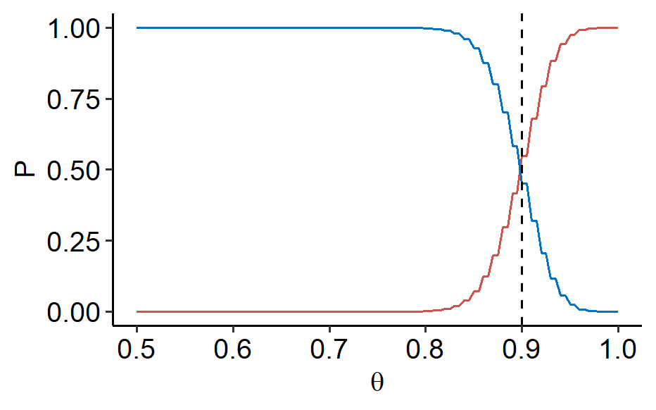
We can see that both functions are continuous of $\theta \in \Theta = [0, 1]$. When $p_1(\theta)$ increases, $p_2(\theta)$ decreases and vice versa. When we make $p_1(\theta) \approx 1$ for $\theta \in \Theta_1$, the continuous $p_2(\theta)$ cannot jump from 0 to 1 when $\theta$ moves across 0.9.
In summary, it’s impossible to always ensure that the correct decision is made. Mistake is inevitable when the true $\theta$ is near the border between $\Theta_1$ and $\Theta_2$, as shown in the figure above1. However, we can introduce a new ingredient: imbalanced severity of false decision. The two mistakes that could be made are
- Choose $H_2$ when $H_1$ is true, and
- choose $H_1$ when $H_2$ is true.
Back to our example, the first mistake means the drug’s effective rate is higher than $90%$, but we didn’t approve it; the second mistake is the effective rate is lower than $90%$, but the drug got approved anyways. The second mistake is more severe.
Such imbalance often arises when $H_1$ corresponds to some new discovery and $H_2$ to some conventional knowledge. Note that such imbalance is not always found in a decision context. Suppose a patients needs to choose the same drug made by two companies, whose true effective rates are $p_1$ and $p_2$, respectively. There is no imbalance of severity of mistake in this decision between $H_1: p_1 < p_2$ vs. $H_2: p_1 > p_2$.
This imbalance leads to the concept of hypothesis testing.
Here’s the R code. Not ideal but it works.
↩︎1 2 3 4 5 6 7 8 9 10library(ggplot2) ggplot(NULL, aes(x = c(0.5, 1))) + stat_function(fun = ~ pbinom(100*., size = 100, prob = 0.9), geom = "line", color = "#CD534C") + stat_function(fun = ~ 1 - pbinom(100*., size=100, prob=0.9), geom = "line", color = "#0073C2") + geom_vline(xintercept = 0.9, linetype = "dashed") + labs(x = expression(theta), y = "P") + ggpubr::theme_pubr()
| Apr 21 | Linear Models | 9 min read |
| Apr 18 | Likelihood Ratio Test | 7 min read |
| Apr 14 | Optimal Tests | 7 min read |
| Apr 09 | p-values | 6 min read |
| Apr 01 | Statistical Test | 13 min read |