p-values
In this section, we make the following assumptions for simplicity:
- $H_0$ is simple, and
- the distribution of test statistic $T$ is continuous.
Therefore, under $H_0: \theta = \theta_0$ with level $\alpha$, we have exactly
$$ \alpha = P_{\theta_0}(T \in RR) $$
Extension beyond these setups is left for more advanced courses. In recent years there’s a collection of articles debating the use of p-values. The concept itself is mathematically sound with no ambiguity, but the problem arises when people who think they understood the meaning of p-values but in fact did not. Our goal in this course is to learn precisely the definition of p-values, and be able to understand and interpret p-values in a correct way in practice.
Motivating example
We start with a motivating example. In the $\alpha$-level Z-test of
$$ H_0: \theta = \theta_0 \quad vs. \quad H_a: \theta \neq \theta_0 $$
and we reject $H_0$ if
$$ |Z| = \left| \frac{\hat\theta - \theta_0}{\hat\sigma} \right| > z_{\frac{\alpha}{2}} $$
However, the information of the magnitude $|Z|$ is lost in this cutoff. Apparently, $|Z|$ being large means the evidence against $H_0$ is significant. We want something that reflects this magnitude. This measure should be independent of the statistical test we’re using, i.e. we want some unified notion that can be used across different tests as an indicator of the significance of the evidence against $H_0$. We’ll be able to use this measure to compare the significance level between different tests.
This value should really be a probability between 0 and 1. In terms of its range, it’s a normalized quantity so that results from different are comparable.
Going back to the example, at level $\alpha$, the rejection region is $RR_\alpha = \{z: |z| > z_{\frac{\alpha}{2}}\}$1. Since $z_\frac{\alpha}{2}$ decreases as $\alpha$ increases, $RR_\alpha$ expands as $\alpha$ increases. In other words, $\alpha$ controls the size of $RR_\alpha$, and the larger the rejection region is, the easier it is to reject $H_0$.
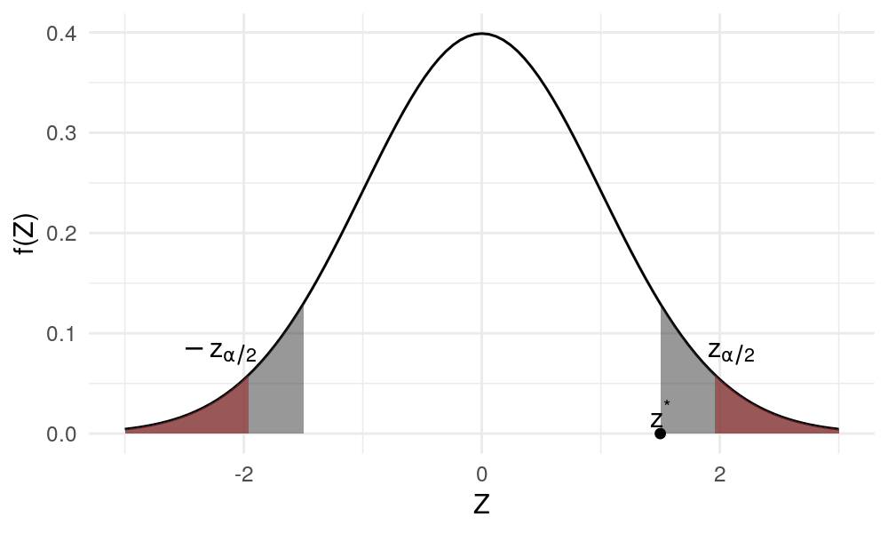
Suppose we observe $Z = z^* > 0$ where $z^$ is fixed. At level $\alpha$, $RR_\alpha$ may or may not contain $z^$. We start with a large enough $\alpha$ such that $RR_\alpha$ includes $z^$, then decrease $\alpha$ until $RR_\alpha$ just excludes $z^$, which is shown as the shaded region in Figure 1. Denote this $\alpha$ as $p$.
More concisely, $p \in (0, 1)$ is the number such that $z^* = z_\frac{p}{2}$. Given the observation $z^*$, $p$ is the smallest possible level where we still reject $H_0$. Note that $H_0$ is rejected whenever $\alpha \geq p$.
If random variable $Z$ is realized at a value other than $z^*$, then the value of $p$ may change.
Definition
To generalize the observations made above, in a hypothesis test, the $\alpha$-level rejection regions $RR_\alpha$ are said to be nested if $RR_\alpha \subset RR_{\alpha’}$ when $\alpha \leq \alpha’$. Namely, the rejection region expands as $\alpha$ increases.
In a hypothesis test with nested rejection regions $RR_\alpha$, the p-value is defined as the random variable
$$ \hat{p} = \min \{\alpha: T \in RR_\alpha \} $$
namely, the smallest possible $\alpha$ such that $H_0$ is still rejected.
Strictly speaking, the “minimum” should be replaced by the “infimum”. Don’t worry about it if you don’t know the difference.
Remark: $\hat{p} = \hat{p}(T)$ is a function of test statistic $T$ (which is random), so $\hat{p}$ is also a statistic. Often we use $p$ to denote an observed $\hat{p}$ when $\hat{p}$ is calculated from an observed sample.
Distribution of the p-value
In a two-sided Z test, we have
$$ \begin{gather*} \hat{p} = \min \{\alpha: T \in RR_\alpha \} = \min\{ \alpha: |Z| > z_\frac{\alpha}{2} \} \\ = \text{The value of } \alpha \text{ which satisfies } |Z| = z_\frac{\alpha}{2} \end{gather*} $$
Note that $\hat{p}$ is random since $Z$ is random. We know $\hat{p}$ is a random variable taking its value in $[0, 1]$. What can be said about its distribution?
Proposition: Under the null $H_0: \theta = \theta_0$, $\hat{p}$ has distribution $Unif(0, 1)$.
Proof: Let $u \in [0, 1]$. Note that
$$ \hat{p} = \min \{\alpha: T \in RR_\alpha \} > u \Leftrightarrow T \notin RR_u $$
Strictly speaking with “inf” replacing “min”, $\hat{p} > u \Rightarrow RR_u$, and $T \notin RR_u \Rightarrow \hat{p} \geq u$, but one can obtain the same conclusion as below.
With this observation that $T$ is not in the rejection region at level $u$, we have
$$ P_{\theta_0}(\hat{p} > u) = P_{\theta_0}(T \notin RR_u) = 1 - u $$
by the definition of the type I error. Hence $P_{\theta_0}(\hat{p} \leq u) = u$, which is the CDF of $Unif(0, 1)$ and the conclusion holds.
This proposition tells us that if the null is true, there should be no bias in the p-value towards any possible value between 0 and 1. This has some important implications, as we will see in the following section.
Another interpretation
This only applies to observed p-values. Suppose $t$ and $t’$ are two possible observed values of test statistic $T$. If the observed p-values $p(t) > p(t’)$, then it means $t’$ is in a smaller rejection region compared to $t$, or $t’$ is a more extreme (unlikely) value than $t$.
Suppose $t$ is an observed value of $T$, and $p = \hat{p}(t)$ is the observed p-value. Then by the proposition above,
$$ P_{\theta_0}(T \text{ is more extreme than } t) = \underbrace{P_{\theta_0}\big( \hat{p}(T) \leq \hat{p}(t) \big)}_{Unif(0, 1)} = \hat{p}(t) = p $$
Hence an observed p-value can be interpreted as the probability of the test statistic being more extreme than the observed value under $H_0$. This is the interpretation that’s often taught in introductory statistics courses. However, we again emphasize that this only applies when we have an observed p-value.
Example
Consider a small-sample test where $Y_i \overset{i.i.d.}{\sim} N(\mu, \sigma^2)$. The hypotheses are
$$ H_0: \mu = \mu_0 \quad vs. \quad H_a: \mu > \mu_0 $$
and the test statistic is $T = \frac{\bar{Y}_n - \mu_0}{\hat\sigma / \sqrt{n}}$. The nested rejection regions are
$$ RR_\alpha = \{t: t > t_\alpha(n-1)\} $$
The p-value is given by
$$ \hat{p} = \min \{ \alpha: T > t_\alpha \} = \alpha \text{ value such that } T = t_\alpha(n-1) $$
Suppose we observed $n=10$ and $T = 2.764$, from which we can calculate $p = 0.01$. Then
$$ P_{\theta_0}(T > 2.764) = 0.01 $$
Meaning that under the null hypothesis, only with $1%$ chance will the $T$ statistic take a value more extreme than the current observed value 2.764.
- ↩︎
1 2 3 4 5 6 7 8 9 10 11 12 13 14 15 16library(ggplot2) ggplot(mapping = aes(x = c(-3, 3))) + stat_function(fun = dnorm, geom = "line") + stat_function(fun = dnorm, geom = "area", xlim = c(-3, -1.96), fill = "red", alpha = 0.5) + stat_function(fun = dnorm, geom = "area", xlim = c(1.96, 3), fill = "red", alpha = 0.5) + stat_function(fun = dnorm, geom = "area", xlim = c(1.5, 3), alpha = 0.5) + stat_function(fun = dnorm, geom = "area", xlim = c(-3, -1.5), alpha = 0.5) + geom_point(aes(x = 1.5, y = 0)) + annotate("text", x = 1.5, y = 0.02, label = "z^'*'", parse = T) + annotate("text", x = 2.1, y = 0.08, label = "z[alpha/2]", parse = T) + annotate("text", x = -2.2, y = 0.08, label = "-z[alpha/2]", parse = T) + labs(x = "Z", y = "f(Z)") + theme_minimal()
| Apr 21 | Linear Models | 9 min read |
| Apr 18 | Likelihood Ratio Test | 7 min read |
| Apr 14 | Optimal Tests | 7 min read |
| Apr 01 | Statistical Decision | 4 min read |
| Apr 01 | Statistical Test | 13 min read |