Bayesian Inference for the Binomial Model

In this lecture we will talk about the same model as in last week, but from a Bayesian perspective. A lot of the details (calculations, choices of priors) are omitted but will be discussed in the next lecture.
Let $A$ be the event of interest from an experiment. Recall that the frequentist view of probability is the limiting relative frequency interpretation:
and the Bayesian takes the “belief” statement:
As we will see, this difference in interpretations has ramifications on how statistical inference is conducted.
The example we use comes from Hoff, Section 3.1. A sample of 129 females aged 65 or older were asked whether or not they were generally happy in the 1998 General Social Survey. Of these, 118 reported being generally happy, while the remaining 11 reported not being generally happy. Some notations:
Our goal is to estimate the true rate $\theta$ of generally happy females aged 65 or older.
Ingredients for Bayesian modeling
Every Bayesian analysis requires specification of the following two pieces:
Sampling model: $p(y \mid \theta)$. This represents how likely is it that we observed $y$ females generally happy in our sample of size $n$, if the true happiness rate is $\theta$? This is going to be identical to how we treat it in the frequentist setting. We’re relating our sample $y$ to the population parameter $\theta$.Prior model: $p(\theta)$ summarizes beliefs associated with different values of the true happiness rate $\theta$, prior to observing data $y$. This doesn’t make sense in the frequentist setting because the parameters would be fixed.
Both of these require us to specify distributions for these models. Once we have the sampling model and the prior model, our goal is to study the posterior distribution denoted $p(\theta \mid y)$. The posterior distribution summarizes beliefs associated with different values of the true happiness rate $\theta$, after observing data $y$. It’s a procedure of updating our prior beliefs in a way that’s consistent with the collected data $y$.
Given the prior and the sampling model, we can compute the posterior by Bayes' theorem:
Here $p(y)$ is the normalizing constant, and we can compute this using just $p(y \mid \theta)$ and $p(\theta)$. In the next few lectures we will focus on posteriors that can be directly computed, but there are complications that arise from this expression which we will get to later.
Sampling model
Let $Y$ be a random variable counting the number of “successes” (e.g. generally happy females) within a sample of size $n$. If $\theta$ represents the true rate of “success” in the population, then an appropriate sampling model is the binomial model:
The probability mass function is
Note this choice is identical to how we would traditionally specify a model, i.e. if we were doing frequentist inference.
Non-informative prior model 1
Suppose we don’t have any real prior beliefs about $\theta$, in other words the only prior belief we have about $\theta$ is that any value between 0 and 1 is equally plausible. An appropriate, non-informative prior model is:
The probability density function of our uniform distribution is
Again, because we are now interpreting probabilities as degrees of belief, it makes sense (and is necessary) to talk about probability distributions for $\theta$, whereas this would have no merit from a frequentist perspective.
Now we can use Bayes’ Theorem to directly compute the posterior distribution. Note that the normalizing constant is
Using the kernel trick1, we will show that the posterior is a beta distribution:
Here we skip the calculations because the uniform prior is a special case of the later beta prior. The beta distribution is a continuous distribution with two parameters, which is defined on the interval from 0 to 1. For our specific data, we have $n = 129$ and $y = 118$, so
Visualizing the model
We can visualize how the observed data updates prior 1 beliefs into posterior 1 beliefs about $\theta$2:
| |
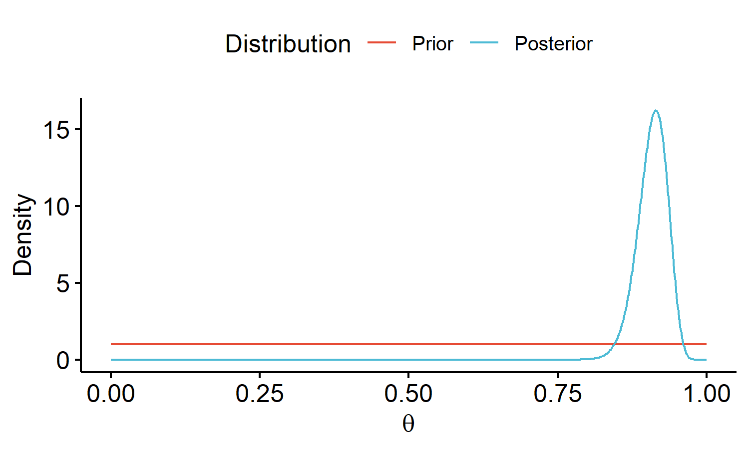
We can see the distribution looks very different. One way to interpret this is our expected true rate of happiness is about 90% based off the observed data. We can also come up with suitable range of values for our guess of $\theta$. We attribute very low degrees of beliefs to values below 80%.
Informative prior model 2
If we think about the previous prior, it might not make sense to say that “only 1% of females are generally happy”. The statement seems implausible even before observing any data, so we might want to specify a different prior distribution.
What if we had knowledge of results from a previous General Social Survey, which identified that 45 of 60 females aged 65 or older were generally happy? An informative prior based on this information may satisfy the following:
- Center: based on this previous study, we might guess $\theta$ is relatively close to $45 / 60 = 0.75$.
- Spread: if 75% is plausible, how much “less plausible” is 76%, i.e. how quickly does the prior distribution go down towards zero? This might depend on the sample size of the previous study – a larger sample size means we might place more trust in the prior beliefs, and that results in less spread in the prior distribution.
An appropriate choice of prior is $\theta \sim Beta(a = 45, b = 15)$ where $a$ and $b$ are hyperparameters. We can choose different hyperparameters3 to adapt to our prior beliefs about $\theta$. In this case, our prior distribution is centered around 75%.
We will show that this choice of sampling and prior model once again results in a beta posterior. Recall from $\eqref{eq:binom-pdf}$ that our sampling distribution $p(y \mid \theta)$ is binomial. The pdf of prior 2 is
where
is the gamma function. Using Bayes’ Theorem, the posterior distribution is
If we look at the denominator, some constant terms that don’t depend on $\theta$ can be taken out of the integral:
Now let $\tilde{a} = y+a$ and $\tilde{b} = n-y+b$, we have
See that the integrand in $\eqref{eq:posterior2-denom-final}$ takes the same form as the pdf of the beta distribution in $\eqref{eq:beta-pdf}$. Thus the entire integral part evaluates to 1, and the denominator is just a constant term. Going back to the posterior model,
So with the informative prior, we have
We can also see that the uniform prior we originally specified is equivalent to a $Beta(a=1, b=1)$ distribution, thus this result is a generalization of what we stated for posterior 1.
Visualizing the model
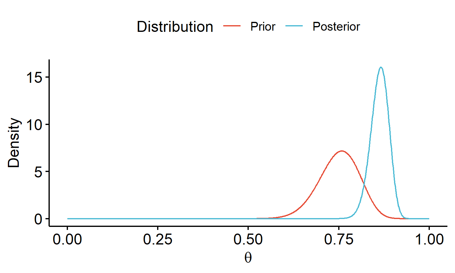
With a slight modification of the code above, we can visualize how the observed data updates our informative prior 2 beliefs into our posterior 2 beliefs about $\theta$:
Shortcut for computing posterior
We compute the posterior distribution via Bayes’ Theorem. Computing the normalizing constant (denominator) is a key part of deriving the posterior. We used the kernel trick to evaluate the integral, by recognizing that the integrand looked like a $Beta(y+a, n-y+b)$ density function.
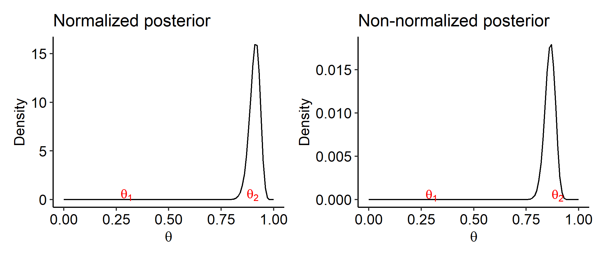
In many cases, the normalizing constant is difficult, if not impossible, to compute directly. But do we actually need to compute this constant? Suppose we are interested in estimating $\theta$ by either $\theta_1=0.3$ or $\theta_2 = 0.9$. Given data $y$, we want to know which value is a better estimate. One way to think about this is we would prefer $\theta_1$ if
This is like a likelihood ratio, but in terms of posterior densities. Note that
does not dependent on the normalizing constant $p(y)$. This means the posterior’s shape only depends on the numerator.
If we plot the true posterior and the numerator side by side, they will be exactly the same shape. $p(y)$ only adjusts how tall the peak is so that the density integrals to 1. We’d prefer $\theta_2$ over $\theta_1$ regardless of which plot we look at.
In light of this, a simpler way to compute the posterior is to work with proportionality statements:
All the colored terms are constant with respect to $\theta$. Thus, the posterior is a $Beta(y+a, n-y+b)$ distribution. We will use this strategy throughout the rest of the course, where instead of evaluating the denominator, we will just focus on proportionality statements with the numerator and see if it looks like a distribution we recognize.
Conjugacy
For the binomial model with a beta prior, we were able to directly recognize the posterior distribution. Sadly this doesn’t always happen. Suppose we specified the following prior model instead:
for some small $\sigma$. This corresponds to the normal distribution that is centered at $\mu$, and $\sigma$ controls the amount of spread. Now if we try to derive the posterior distribution,
This is no longer the kernel of some distribution that we recognize. This doesn’t mean our prior belief or the sampling model is wrong. We’d still get a valid posterior distribution, but we won’t be able to find the normalizing constant in closed form. In later lectures we’ll talk more about how to handle situations like this.
The prior $\theta \sim Beta(a, b)$ was conveniently chosen because we obtain a closed-form posterior distribution. This choice of convenience is known as a conjugate prior. Formally speaking, let $\mathcal{F}$ be the class of sampling models $p(y \mid \theta)$ and $\mathcal{P}$ be the class of prior distributions $p(\theta)$. We say the prior class $\mathcal{P}$ is conjugate for sampling model class $\mathcal{F}$ if:
Intuitively, the prior $p(\theta)$ and posterior $p(\theta \mid y)$ come from the same family of distributions. For example, in the binomial model we have
We can say the beta prior is conjugate for the binomial model, since our posterior is also beta-distributed.
Pros and Cons
Pros to conjugate prior specification:
- Allows direct computation of posterior, i.e. a closed-form, recognizable posterior distribution.
- Easy to understand and very interpretable.
- Good starting choice.
Cons to conjugate prior specification:
- Now always available for every model, particularly if $\theta$ consists of a large number of parameters (high-dimensional).
- Restrictive in terms of modeling choices. It might not always be the choice which best reflects prior beliefs about $\theta$.
Numerical posterior summaries
It is useful to produce numerical summaries of the posterior distribution:
Measures of center
First, we focus on measures of center. The posterior mean tells us what is the expected proportion of generally happy females aged 65 or older, given the observed data.
The equation above can be interpreted as a weighted sum of the prior mean for $\theta$ and the observed sample proportion. The boxed terms are weights on the prior mean and the observed data, respectively.
The posterior mean is a weighted sum of the prior mean and the sample mean. As the sample size $n \rightarrow \infty$, $E(\theta \mid y) \rightarrow y/n$, i.e. the data “overrides” the prior information.
An alternative measure of center is the maximum a posteriori (MAP) estimate. This is also known as the posterior mode, and tells us what is the most likely proportion of generally happy females aged 65 or older, given the observed data4.
For our posterior,
We might report the MAP estimate over the posterior mean because the MAP is the value of $\theta$ for which our posterior beliefs are highest. This is especially useful for skewed distributions.
Measures of variation
We may also be interested in the amount of variation in the posterior of $\theta$. The posterior variance measures how much uncertainty there is in the proportion of generally happy females aged 65 or older, given the observed data.
As the observed sample size $n$ increases, the posterior variation decreases. This measure however does not have the nice interpretation the posterior mean has. A better way to quantify uncertainty in our posterior beliefs about $\theta$ is by computing a range of values for which it is likely $\theta$ falls within.
A $100(1-\alpha)\%$ posterior credible interval for $\theta$ is determined by endpoints $l(Y)$ and $u(Y)$ which satisfy
This is saying the posterior probability that $\theta$ is in the interval $[l(Y), u(Y)]$ is equal to $1-\alpha$. This is actually a really nice interpretation because all we need to do is to find the two endpoints on the posterior distribution which we directly have.
Note that this is not the same as a confidence interval! A $100(1-\alpha)\%$ confidence interval for $\theta$ would satisfy
The frequentist CI works regardless of what sample we took from the population. More specifically, it is not conditional on the specific observed data because it’s based off repeatedly generated data from the population. That being said, credible intervals and confidence intervals often coincide with each other. In the Bayesian setting, we always report credible intervals.
Types of credible intervals
Now the question is how do we select $l(Y)$ and $u(Y)$. There are two different ways to construct intervals by determining these endpoints: a percentile-based interval, or a highest posterior density (HPD) region.
Percentile-based interval
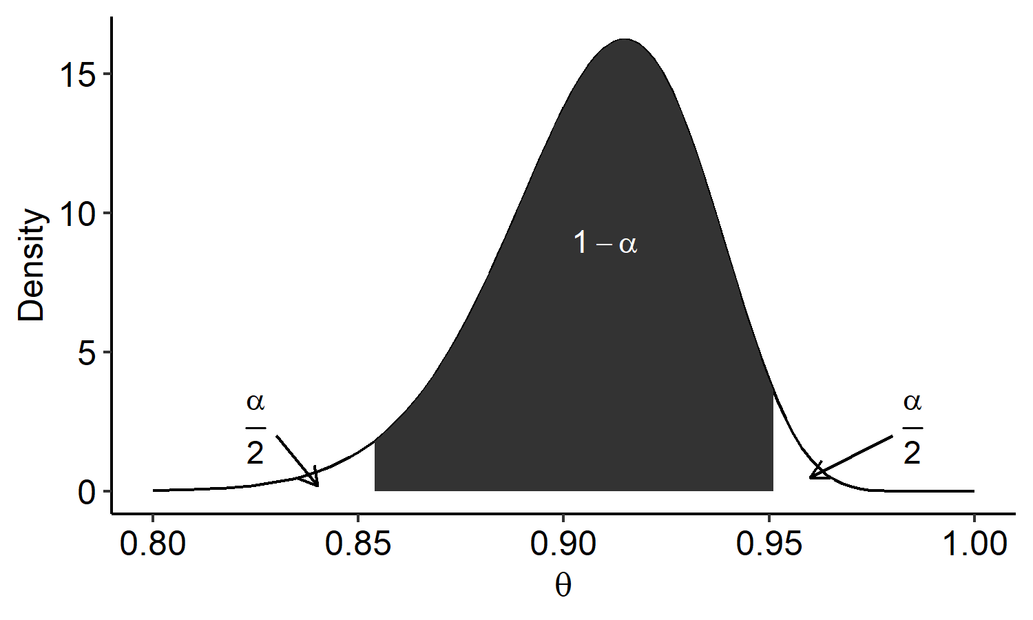
If we choose $l(Y)$ and $u(Y)$ as percentiles of the posterior, then we will have $\eqref{eq:credible-interval}$. We want $1-\alpha$ in the shaded region. Choosing percentiles means we want $\frac{\alpha}{2}$ probabilities in the left and right tails. The cutoff points can be found by
The numbers are found in R using the qbeta() function. For example, the 2.5-th percentile $l(Y)$ can be found by qbeta(0.025, y+1, n-y+1). We could say that with probability 0.95, the true rate $\theta$ is between 0.854 and 0.951. This is a much more straightforward interpretation than the frequentist interpretation of confidence intervals.
HPD region
The percentile-based interval is easy to compute and is most commonly used. However, some values of $\theta$ outside of a percentile-based CI might have higher posterior densities than the values within (due to the “asymmetry”).
The HPD region is constructed in a way to resolve this issue. $l(Y)$ and $u(Y)$ are chosen to satisfy:
- $P(l(Y) < \theta < u(Y) \mid Y=y) = 1-\alpha$.
- Any value of $\theta$ between $l(Y)$ and $u(Y)$ must have higher posterior density than values outside the interval.
In R, the HDInterval::hdi() function can be used to find the HPD region. As a comparison to the 95% percentile CI of (0.854, 0.951), the HPD region is (0.858, 0.955). In this case the two are not very different because the posterior is quite symmetric, but the HPD region comes handy when the posterior is skewed or multimodal.
Comparing the two posteriors
Now we can summarize and compare posteriors 1 and 2:
| Posterior | $\theta \mid y \sim Beta(119, 12)$ | $\theta \mid y \sim Beta(163, 26)$ |
|---|---|---|
| Posterior mean | 0.908 | 0.862 |
| Posterior variance | 0.0006 | 0.0006 |
| MAP | 0.915 | 0.866 |
| 95% posterior CI | (0.854, 0.951) | (0.810, 0.908) |
Posterior 2 is shifted to the left of 1, since we specified an informative prior which was centered around $\theta = 0.75$. Both posteriors are concentrated on a small set of values.
Sensitivity analysis
Re-visiting our prior specification, suppose we believed from past studies that the true rate of generally happy females aged 65 or older was closer to 75%. Consider the conjugate prior for $\theta$ ($\theta \sim Beta(a, b)$), with the following hyperparameter choices:
| Prior | “Prior” sample size | $a$ | $b$ |
|---|---|---|---|
| 1 | 2 | 1 | 1 |
| 2 | 4 | 3 | 1 |
| 3 | 60 | 45 | 15 |
| 4 | 120 | 90 | 30 |
Recall that the prior mean of $\theta$ is $E(\theta) = a/(a+b)$. We can interpret $a$ as the “prior” number of successes, and $b$ as the “prior” number of failures. We can control $a$ and $b$ so that the prior mean is centered around 0.75. If we increase the prior sample size, we put more emphasize on the prior beliefs.
In the table above, prior 1 is the non-informative prior, and the other three are centered at $\theta = 0.75$. The posterior distribution under these prior choices are:
A study of how sensitive the posterior is to our prior assumptions is called a sensitivity analysis. We’re looking at how sensitive is our posterior distribution to different reasonable choices of prior distributions, and it is remarkably important for any Bayesian analysis.
As we go from (1) to (4), we place more emphasis on our prior beliefs. The 95% HPD credible intervals for $\theta$ are:
| Prior | Credible interval |
|---|---|
| (1) | (0.858, 0.955) |
| (2) | (0.860, 0.955) |
| (3) | (0.813, 0.910) |
| (4) | (0.789, 0.880) |
The first two are very similar to each other due to their small sample sizes. As the sample size increases, the CIs shift to the left. The take-away message is if one does not have any prior information, using a non-informative prior to “let the data drive inference” is a good choice. If one does have prior information, use it carefully especially if the posterior is sensitive to the choice of prior, i.e. if there’s not much observed data.
Concluding remarks
- Every Bayesian analysis proceeds in a similar fashion to this one. In the coming lectures, we will talk more about different details associated with this process.
- Neither posterior nor 2 should be deemed correct or incorrect. It all depends on the amount of prior information available. In this example, the posterior was quite different between the two prior choices. It is often beneficial to study how sensitive the posterior is to prior information.
- Generally, the prior distribution should not depend on the observed data. This is often referred to as “double-dipping”, and can lead to faulty conclusions due to over-reliance on the data. You can base the prior off previous studies, scientific knowledge, or other intuition.
After writing out the posterior distribution using Bayes’ Theorem, we make the denominator look like the integrals of a pdf of some known distribution so that we don’t have to solve it. ↩︎
When we report Bayesian results, it’s always good to plot the prior and posterior simultaneously because this gives us all the information about our beliefs about $\theta$ before and after observing the data. ↩︎
In this specific case, the prior hyperparameters have nice interpretations: $a$ is the prior number of successes, $b$ is the prior number of failures, and $a+b$ is the prior sample size. ↩︎
This value corresponds to the peak in the plot of the posterior density function. ↩︎
| Apr 26 | A Bayesian Perspective on Missing Data Imputation | 11 min read |
| Apr 19 | Bayesian Generalized Linear Models | 8 min read |
| Apr 12 | Penalized Linear Regression and Model Selection | 18 min read |
| Apr 05 | Bayesian Linear Regression | 18 min read |
| Mar 29 | Hierarchical Models | 18 min read |